

Yes, we're now running our only Summer Sale. All Courses are 30% off until 20th July, 2026:
Learn through the super-clean Baeldung Pro experience:
>> Membership and Baeldung Pro.
No ads, dark-mode and 6 months free of IntelliJ Idea Ultimate to start with.
1. Overview
In this tutorial, we’ll explore the binary search tree (BST) data structure.
First, we’ll start with an overview of how the BST works and when to use it, and then we’ll implement the fundamental operations of lookup, insertion, and traversal.
2. Binary Search Trees
Simply put, a binary search tree is a data structure that allows for fast insertion, removal, and lookup of items while offering an efficient way to iterate them in sorted order.
For these reasons, we use binary search trees when we need efficient ways to access or modify a collection while maintaining the order of its elements.
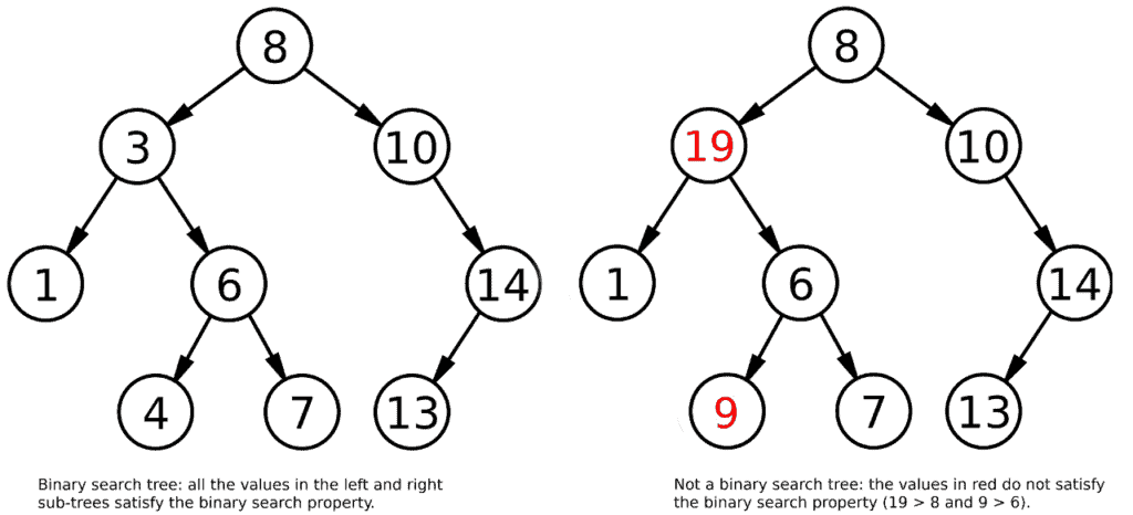
The fundamental feature of a binary search tree, as opposed to a simple binary tree, is that it satisfies the binary search property. This property states that, for each node, its value must be less than the values in the right sub-tree and greater than those in the left sub-tree:
As a result, lookup, insertion, and removal operations have a complexity of  . The reason for this is that, when traversing the tree from root to leaf, we can discard half of the tree at each step, according to the input value being greater or less than the one in the current node.
For example, if we want to see if the tree on the left contains the value 9, we already know that we’ll only have to look in the right sub-tree of the root node, because 9 is greater than 8, the value of the root.
2.1. Lookup
Lookup on a binary search tree is performed by traversing the tree down from the root and by choosing, at each step, if we want to continue by going right or left. We repeat this process until we find our value or the current node doesn’t have a right/left child.
This is an implementation using recursion:
algorithm lookup(tree, key):
    // INPUT
    //   tree = a binary search tree
    //   key = the key to look for
    // OUTPUT
    //   true if the key is found, false otherwise

    if key = tree.key:
        return true

    if key < tree.key:
        if not tree.hasLeftChild():
            return false

        return lookup(tree.leftChild(), key)

    if key > tree.key:
        if not tree.hasRightChild():
            return false

        return lookup(tree.rightChild(), key)
2.2. Insertion
When inserting an element in the tree, we first need to find the correct position to place it in, because the tree has to still satisfy the binary search property.
The algorithm ends up being very similar to the lookup operation, with the difference being that we create a new node, instead of returning false, when the current node has no child:
algorithm insert(tree, key):
    // INPUT
    //   tree = a binary search tree
    //   key = the key to insert
    // OUTPUT
    //   a binary search tree with a new node for the key,
    //   or the same input tree if the key already exists

    if key < tree.getKey():
        if tree.hasLeftChild():
            insert(tree.getLeftChild(), key)
        else:
            tree.setLeftChild(key)

    else if key > tree.getKey():
        if tree.hasRightChild():
            insert(tree.getRightChild(), key)
        else:
            tree.setRightChild(key)
2.3. Traversal
Trees are non-linear data structures, meaning that an ordering of their elements is not defined by default. Instead, we can access its elements in different orders by using different traversal algorithms.
Obtaining the elements in ascending order is easily implemented in the context of a BST, as we simply need to perform depth-first in-order traversal:
algorithm dfs(tree):
    // INPUT
    //   tree = a binary search tree
    // OUTPUT
    //   the function prints the tree's values in depth-first in-order

    if tree.hasLeftChild():
        dfs(tree.getLeftChild())

    print(tree.value)

    if tree.hasRightChild():
        dfs(tree.getRightChild())
Conversely, if we want to visit the elements in descending order, we have to use reverse in-order traversal. To do this, we’ll simply start our depth-first search on the right sub-tree. In practice, we just need to invert the references to  and
and  in our
  algorithm.
This operation has a time complexity of  – because there are
  nodes in the tree and each one of them is only visited once.
3. Conclusion
In this quick article, we explored the basics of how binary search trees work and why they can be quite useful.
We’ve also seen how to find and insert elements, and how to print them in ascending or descending order using depth-first in-order or reverse in-order traversal.