

Learn through the super-clean Baeldung Pro experience:
>> Membership and Baeldung Pro.
No ads, dark-mode and 6 months free of IntelliJ Idea Ultimate to start with.
Last updated: March 18, 2024
Learn through the super-clean Baeldung Pro experience:
>> Membership and Baeldung Pro.
No ads, dark-mode and 6 months free of IntelliJ Idea Ultimate to start with.
In Data Science, one of the first phases of discovery is determining what is in the data. The less we know about the data, the more we need algorithms that will help us discover more about it. If we graph our data and can see well-defined clusters, then we’ve got algorithms where we simply supply the numbers of clusters ourselves.
But, if we have a large number of parameters or less well-defined clusters, it’s more difficult to use an algorithm that requires a number of clusters up-front. Luckily, there are a number of algorithms that don’t require that we have that up-front knowledge. In this tutorial, we’ll discuss some of those algorithms.
Clustering is similar to classification. To classify, we need to know into what categories we want to put the data. But, we can use clustering when we’re not sure what those classifications might be. In that case, it’s up to the algorithm to find the patterns and to create the clusters. Different algorithms will produce different clusters. So, it’s not uncommon to use more than one algorithm and find different patterns, or clusters, from each.
We use the term cluster because we imagine doing this on a graph, where we can see the points clustered together. What is a cluster? It’s a group of points that are close to each other:
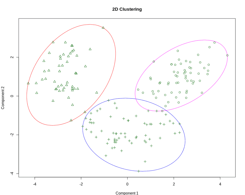
But how do we determine that they are “close”? We measure the distances between them.
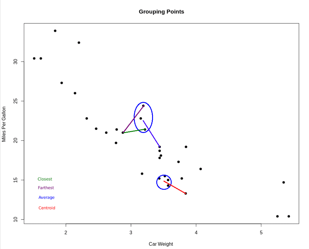
Simply put, there are four methods we can use for deciding “how close” a cluster and a nearby point might be:
Once we determine what distance we want to measure, how do we measure it? In basic geometry, we learned the Euclidean Distance Formula:

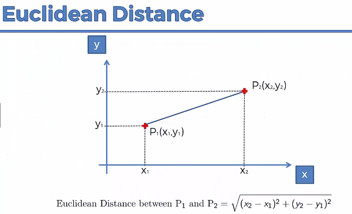
And this appears to be the most common method used, but there are a number of other options.
Having decided how to define the distance and what formula we’ll use, we’re ready to select a clustering algorithm.
There are a number of ways of achieving clustering:
And there are a number of ways of classifying clustering algorithms: hierarchical vs. partition vs. model-based, centroid vs. distribution vs. connectivity vs. density, etc. Each algorithm determines whether one data point is more “like” one data point than it is “like” another data point. But how that likeness is determined differs by the algorithm implemented. Let’s do a quick survey of some of the algorithms available, focusing on those that do not require that we define the number of clusters up-front.
Hierarchical clustering is a hierarchical algorithm that uses connectivity. There are two implementations: agglomerative and divisive.
In agglomerative clustering, we make each point a single-point cluster. We then take the two closest points and make them one cluster. We repeat this process until there is only one cluster.
The divisive method starts with one cluster, then splits that cluster using a flat clustering algorithm. We repeat the process until there is only one element per cluster.
The algorithm retains a memory of how the clusters were formed or divided. This information is used to create a dendrogram. The dendrogram is used to set the thresholds for determining how many clusters should be created.
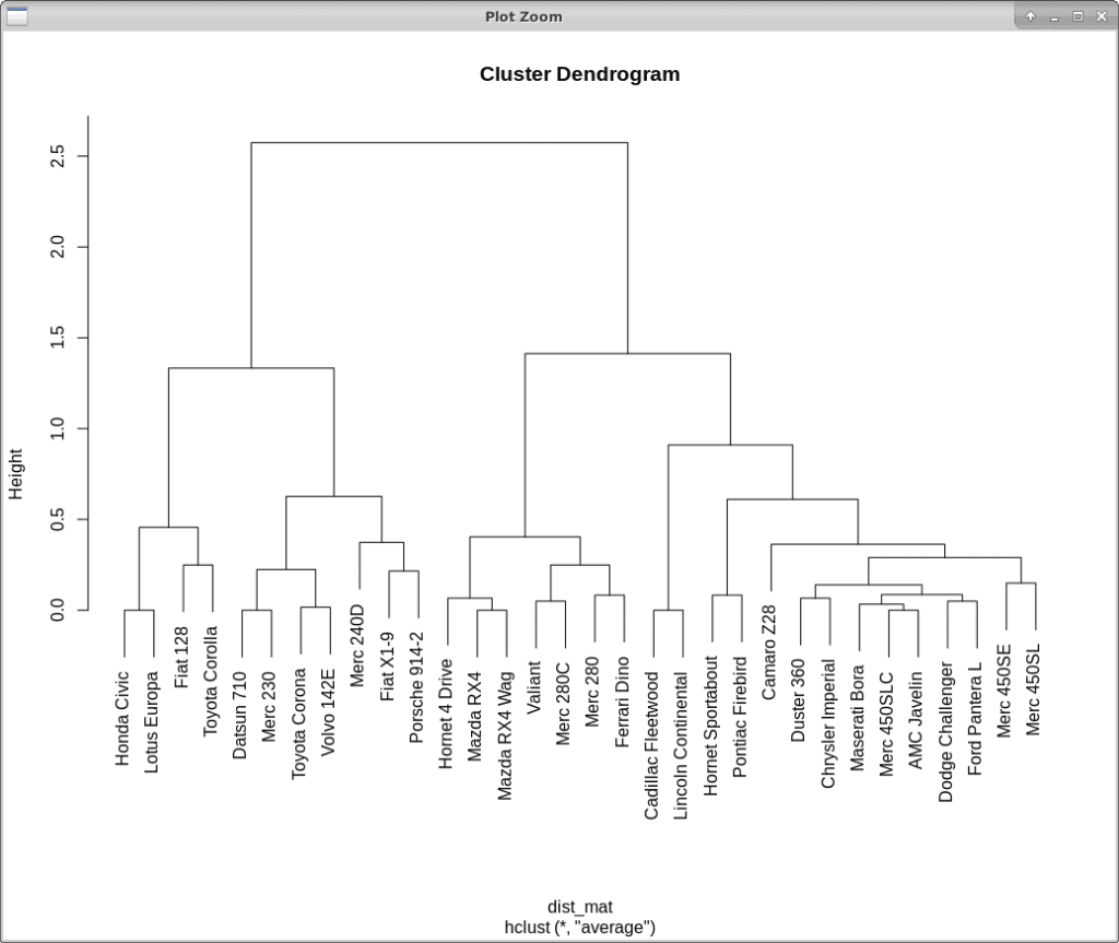
We find the optimal number of clusters by finding the longest unbroken line in the dendrogram, creating a vertical line at that point, and counting the number of crossed lines. In the example above, we find 2 clusters.
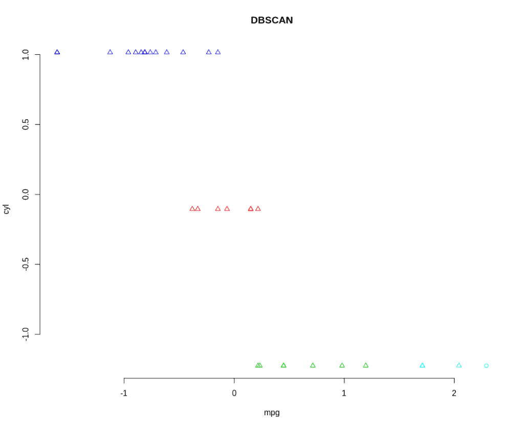
DBSCAN is a density-based clustering algorithm. It groups together points within a distance measurement using a minimum-point-count threshold.
EPS (epsilon) is the maximum radius of the neighborhood. It defines how far apart the points can be to be considered part of the cluster. We don’t want this value to be too small since it will be difficult to find the minimum number of points in the given region. If the value is too large, a majority of the objects will be in one cluster.
The MinPts is the minimum number of points to form a dense region. We can calculate this value from the number of dimensions in the dataset. The rule of thumb is:

The minimum value allowed is 3. But for larger datasets or datasets with a lot of noise, a larger value is better.
Mean-shift is a centroid-based algorithm. It works by updating candidates for centroids to be the mean of the points within a given region. That is, it’s looking for the densest regions and finding their centroids.
To implement mean-shift, we initialize a random seed and a window (W). Then, we calculate the center of gravity (the mean) of W. We shift the search window to the mean, then repeat the calculation until convergence is achieved:
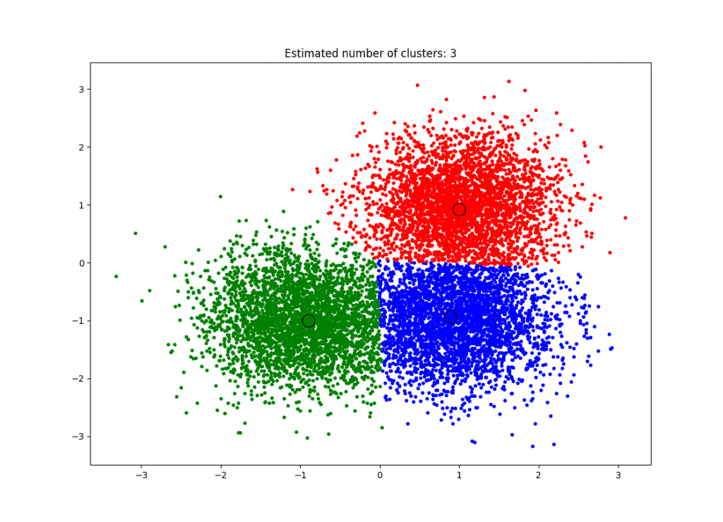
Final mean shift clustering, with centroids and clusters defined.
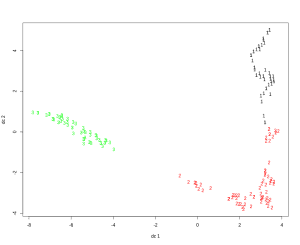
In spectral clustering, data points are treated as nodes on a graph. The nodes are mapped to low-dimensional space that can be easily segregated to form clusters. Unlike other algorithms, which assume a regular pattern, no assumption is made about the shape or form of the clusters in spectral clustering.
In order to find the clusters, we first create a graph. This graph can be represented by an adjacency matrix, where the row and column indices represent the nodes, and the entries represent the presence or absence of an edge between the nodes. We then project this data onto a lower-dimensional space and create the clusters:
In this article, we have shown how clustering algorithms are defined and differentiated.
We’ve shown different examples of the types of algorithms that can be used when we don’t know how many clusters there will be. Once we determine how many clusters there will be, we can use the K-Means Clustering algorithm to gain more insight into our data.
Clustering is just one exploratory algorithm for data analysis. And data exploration is just one step in the data science process. For insight into a tool that helps with the entire process, check out our guide to Spark MLlib.