

Learn through the super-clean Baeldung Pro experience:
>> Membership and Baeldung Pro.
No ads, dark-mode and 6 months free of IntelliJ Idea Ultimate to start with.
Learn through the super-clean Baeldung Pro experience:
>> Membership and Baeldung Pro.
No ads, dark-mode and 6 months free of IntelliJ Idea Ultimate to start with.
One of the main problems in machine learning and data science is how to represent different data types. Typically, we encode data like text and images as a vector or a matrix so the computer can understand and process them. However, the larger and more complicated data urgently need a more computational and memory-efficient method to obtain a dense and meaningful representation. Hence, the concepts of ‘latent space’ and ’embedding space’ come into play.
‘Latent space’ and ‘Embedding space’ are vector spaces that help us obtain the essence of our data without getting lost in other unnecessary information.
In this tutorial, we’ll explore and compare these two concepts.
Latent space is a compressed, lower-dimensional space into which high-dimensional data transforms. Projecting a vector or matrix into a latent space aims at capturing the data’s essential attributes or characteristics in fewer dimensions.
Consider a photograph. For us, it is a vivid image. In contrast, a computer sees it as a large matrix of pixel values. In order to capture the critical feature of the photo, such as the main subject, we transfer the original pixel matrix into a latent space. The new matrix will be smaller in size than the original one. Meanwhile, the reducing dimensions help filter the unwanted information in the photo.
There are several approaches to compressing data into a lower-dimensional space, such as a statistical method called principle component analysis (PCA) as well as a deep learning autoencoder.
PCA is a statistical method used to reduce the dimensionality of data. It identifies the principal components in the dataset that maximized variance. The first principal component is the direction in which the data varies the most. By selecting the top k principal components, we can reduce the data from n dimensions to k dimensions.
Typically, while applying PCA, we normalize the data such that it has a mean of zero and a standard deviation of one. Then, we calculate the covariance matrix of the data, which ranges to capture the inner product between features. After that, we compute the Eigenvalues and Eigenvectors of the covariance matrix. These Eigenvectors (principal components) determine the new feature space.
Latent space is especially useful in deep learning, especially with autoencoders. For instance, when handling images, the autoencoder reduces the image to a few key points in this latent space.
An autoencoder is a neural network with two parts: an encoder and a decoder. As the name says, the encoder encodes the input data into a latent space. On the other hand, a decoder attempts to reconstruct the encoded data from the original input.
The diagram below illustrates a standard autoencoder:
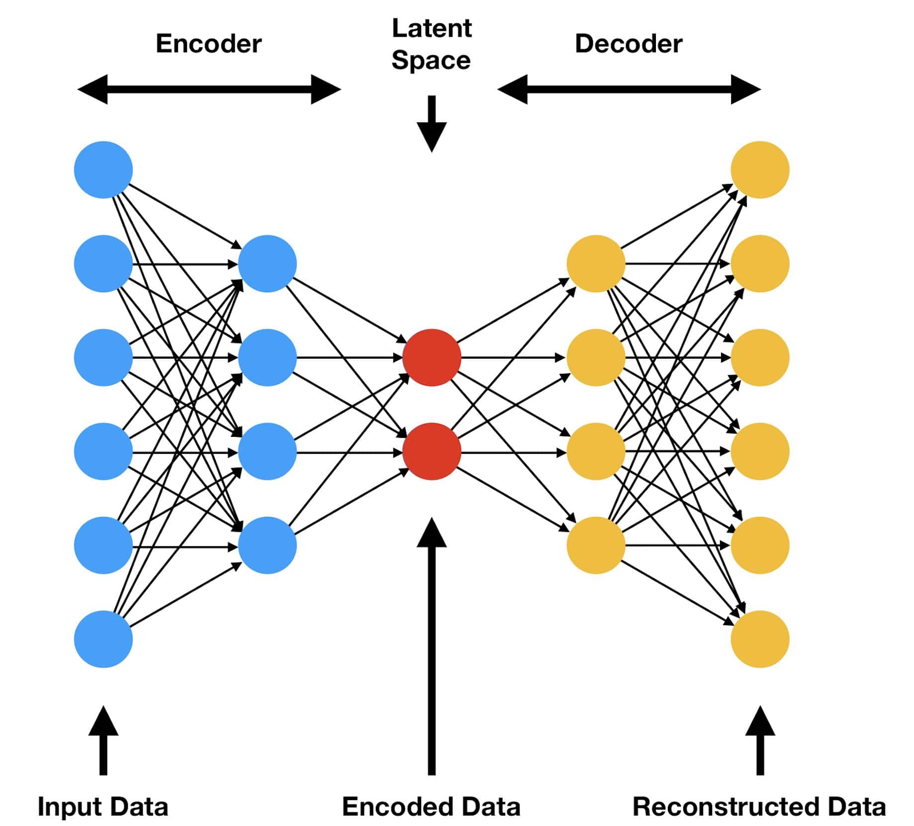
During training, the autoencoder minimizes the difference between the input and the output, usually by using a form of the mean square error. After training, we consider the encoded representation in the latent space as a compressed form of the original data.
There are various specialized forms of autoencoders, such as Variational Autoencoders (VAEs), Sparse Autoencoders, and Denoising Autoencoders. Each of them contains unique properties and applications.
Imaging we want to work as a vector, where each value within the vector counts the word occurrence within a document:
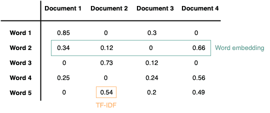
However, a large-scale dataset usually contains numerous words and documents. For some words, it might only appear in a small group of documents. Therefore, their vector representations are sparse, and the values are mostly ‘0’. A space representation can cause various challenges in machine learning, such as memory consumption and computational efficiency.
To solve this, we can compress the representations into a latent space. By contrast, we can apply a more efficient way, embedding, in this case. Embedding space is where data of various types (words, users, movies, etc.) get represented as vectors to capture their relationships and semantic meaning.
Thus, we can apply word embeddings to represent a word, where words with similar meanings are mapped to nearby points in the embedding space. With word embedding, words like ‘king’ and ‘queen’ would be closer in this space than ‘king’ and ‘apple’.
For instance, the figure below shows the word embeddings in a 3-dimensional space:
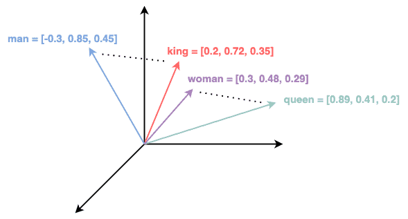
By projecting the data item into an embedding space, it translates complex relationships or features into distances and angles in this space. As a result, we can compare these items using algebra.
Embedding is heavily used in Natural Language Processing and recommendation systems.
Typically, we use text embedding in Natural Language Processing to represent words/sentences in a dense vector space. In such a way, the words/sentences with similar meanings or appearing in similar contexts are closer to each other in this pre-defined vector space. There are several classic algorithms and techniques to generate word embeddings, for example, Word2Vec, Glove, FastText, etc.
A classic word embedding model learns a mapping function to project the word into a certain vector space using the co-occurrence relationship between words. After learning the mapping function, they assign a fixed embedding to each word.
In the meanwhile, with the advent of Transformer models like BERT (Bidirectional Encoder Representations from Transformers), the concept of word embeddings has evolved to contextualized word embeddings. Unlike traditional word embeddings mentioned before, contextualized embeddings provide word representations that depend on the surrounding context. This means the word ‘Java’ would have different embeddings for the programming language and coffee.
User and item embeddings are common in recommendation systems. Users and products (like movies or books) are represented in an embedding space. The system can make personalized recommendations by observing which items are close to a particular user in this space.
In a movie recommendation system, like IMDB, the website recommends different movies to each user based on their ratings. One basic approach to embedding users and movies starts with randomizing embedding for the users and movies. The system gives an estimate of the user’s rating for certain movies based on the dot product between the user and movie embeddings. In the meanwhile, the algorithm minimizes the error between the actual rating and the predicted rating.
After training on many user-movie interactions, the embeddings capture the underlying factors that influence user ratings. For instance, factors might include movie categories like action or drama, themes like love or war, or any abstract concept that consistently influences ratings. On the other hand, user embedding could capture factors such as demographics.
Even though both latent space and embedding space involve reducing high-dimensional data into a lower dimension, they serve different purposes and have different usages.
Latent space aims at capturing essential features in a compressed form. Therefore, models like autoencoder and PCA are widely used for data compression and noise reduction.
Alternatively, an embedding space targets representing data in a way that captures semantic relationships. For that reason, it is common in dealing with categorical data or Natural Language Processing and recommendation systems.
The effectiveness of a machine learning model can be significantly impacted by the dimensions chosen for both latent space and embedding space. The dimensions provide the number of variables or features used to represent the data.
Since latent space is about representing data compactly, we chose its dimensions based on the level of compression required. Though a wider latent space might be able to catch more data, it also requires more data in order to train properly.
However, the dimension of an embedding space often depends on the complexity of the relationships to be captured. The ideal dimensionality relies on a number of variables, including the size of the training dataset, the available computing power, and the particular task at hand.
Some simple models like PCA can be interpreted while generating latent space.
However, when leveraging deep learning approaches, both latent space and embedding space may not always be easily interpretable.
Like latent space, some embedding methods, such as Word2Vec, are interpretable, with distances and angles representing relationships or similarities. Yet, the development of deep learning and Transformer-based approaches also increases the challenge of interpreting the features captured by the embeddings.
In this article, we dived into the concept and application of latent space and embedding space.
While both latent and embedding spaces are able to represent high-dimensional data in a reduced form, they serve distinct purposes and have different applications. Latent space focuses on compression and capturing essential features. Nevertheless, embedding space focuses more on capturing relationships and semantics.
These two approaches also share some similarities. The dimension of the latent and embedding space is crucial to the model’s performance. In addition, the new vector can be difficult to interpret depending on the approaches leveraged for creating the vector space.