Learn through the super-clean Baeldung Pro experience:
>> Membership and Baeldung Pro.
No ads, dark-mode and 6 months free of IntelliJ Idea Ultimate to start with.
Last updated: February 13, 2025

Learn through the super-clean Baeldung Pro experience:
>> Membership and Baeldung Pro.
No ads, dark-mode and 6 months free of IntelliJ Idea Ultimate to start with.
Information theory is a scientific field of great interest as it is expected to provide answers for today’s data storage and data analysis problems. It is this field that provides the theoretical base for data compression, after all. There are purely statistical approaches but machine learning offers flexible neural network structures that can compress data for a variety of applications.
In this tutorial, we’ll discuss the function, structure, hyper-parameters, training, and applications of different common autoencoder types.
There are many ways to compress data and purely statistical methods such as principal component analysis (PCA) can help identify the key features accountable for the variability in the data and use these to represent the information using fewer bits. This type of compression can be called “Dimensionality Reduction”. However, this PCA solution can only offer an encoding with linearly uncorrelated features.
The machine learning alternative solution proposes neural networks that are structured as autoencoder models. Autoencoders can learn richer, non-linear encoding features. These features can correlate with each other and are therefore not necessarily orthogonal to one another. Using these functions we can represent complex data in a latent space.
For example, when discussing Convolutional Neural Networks (CNNs) for facial recognition, these can be used as autoencoders for image data. They can allow a user to store photos using less space by encoding the image by lowering the quality just a little bit. The difference or loss in quality between the output and input images is called reconstruction loss.
The main goal for autoencoders is to represent complex data using as little code as possible with little to no reconstruction or “compression” loss. To do so, the autoencoder has to look at the data and construct a function that can transform a particular instance of data into a meaningful code. We can think of this as a remapping of the original data using fewer dimensions. We can also keep in mind that this code has to be interpreted later on by a decoder to access the data.
To better understand the functioning of these models, we’ll decompose them into individual components. We’ll describe the structure in the same order that the data travels our neural net, discussing encoders first, then the bottleneck or “code” and then decoders. These segments of autoencoders can be seen as different layers of nodes in a model. The image below helps interpret these three different components. The arrow indicates the flow of the data in our model:
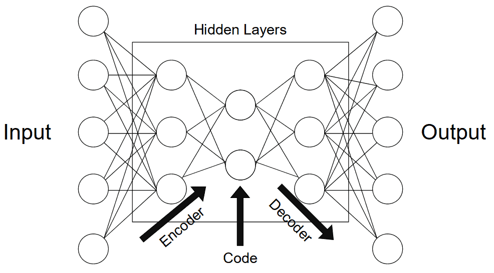
The encoder’s role is to compress the data into a code. In neural networks, we can implement this phenomenon by connecting a series of pooling layers, each one reducing the number of dimensions that are present in the data. In doing this, we can de-noise data by keeping only the parts of it that are relevant enough to encode.
The layer of the neural network that has the fewest dimensions, generally in the middle of all the layers, is called the bottleneck. If we’re interested in keeping more information about a specific instance, we’d need a larger code size. This “code size” hyper-parameter is important as it defines how much data gets to be encoded and simultaneously regulates our model. A very big code will represent more noise but too little code may not accurately represent the data at hand.
The decoder component of the network acts as an interpreter for the code. In the case of convolutional neural nets, it can reconstruct an image based on a particular code. We can think of this component as a value extraction, interpretation, or decompression tool. Image segmentation is usually the decoders’ job as well. If we keep our last example of classifying dog pictures, we could continue decoding while adding a copy of previous compressed layers to each layer of decoder nodes. In doing so, we should obtain a photograph with a subset of pixels that identify the dog in the picture and segment it from the background and other objects.
Generative models such as Variational Auto-Encoders (VAEs) can even use the decoder to render data that doesn’t exist. This can be useful for data augmentation purposes. In having diverse data sets from generative models, other models can learn more thoroughly from data.
Autoencoders are applied in many different fields across machine learning and computer science. Here are the main types that we can encounter and their respective common applications.
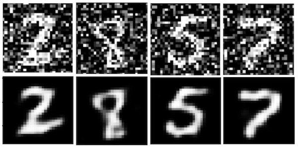
These types of autoencoders are meant to encode noisy data efficiently to leave random noise out of the code. In doing so, the output of the autoencoder is meant to be de-noised and therefore different than the input. We can see what an implementation of this would look like using the popular MNIST dataset, as presented in the image below:
These types of autoencoders can be used for feature extraction and data de-noising.
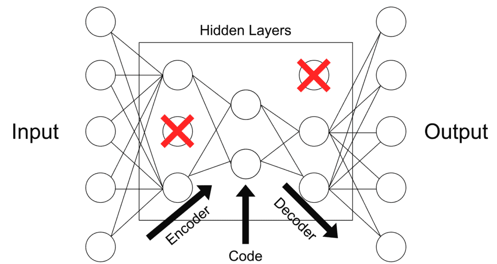
This type of autoencoder explicitly penalizes the use of hidden node connections. This regularizes the model, keeping it from overfitting the data. This “sparsity penalty” is added to the reconstruction loss to obtain a global loss function. Alternatively, one could just delete a set number of connections in the hidden layer:
This is more of a regularization method that can be used with a broad array of encoder types. Applications may vary.
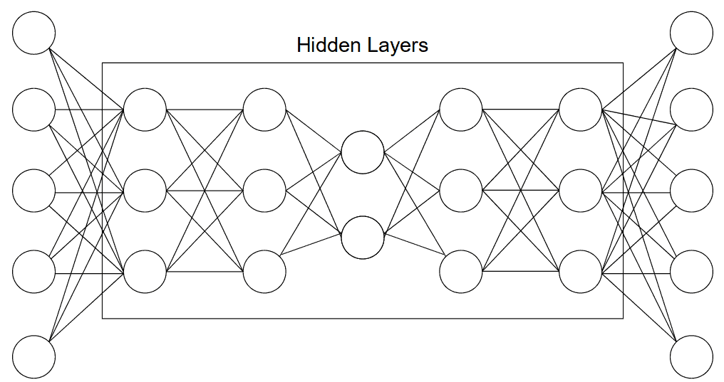
Deep autoencoders are composed of two symmetrical deep-belief networks. This structure is similar to the “general structure” representation of an autoencoder using nodes and connections found above. These mirrored components can be described as two restricted Boltzmann machines acting as encoders and decoders:
Autoencoders of this type are used for a wide array of purposes such as feature extraction, dimensionality reduction, and data compression.
Contractive autoencoders penalize big variations in code when small changes in the input occur. This means that similar inputs should have similar codes. This usually means that the information captured by the autoencoder is meaningful and represents a large variance in the data. To implement this, we can add a penalty loss to the global loss function of the autoencoder.
Data augmentation is a great type of application for these types of autoencoders.
These autoencoders have smaller hidden dimensions in comparison to input. This means that they excel at capturing only the most important features present in the data. These types of autoencoders usually do not need regularization as they do not aim to reproduce outputs similar to inputs but rather rely on the compression stage to capture meaningful features in the data:
Feature extraction is the main type of application for this type of autoencoders.
Convolutional autoencoders can use a sum of different signals to encode and decode. The most common version of this is probably a U-Net convolutional model. This model developed for biological imaging applications will interpret the output of different filters across an image to classify and ultimately segment the image data. Similar convolutional models are used today to segment images.
Applications are found for these autoencoders in computer vision and pattern recognition.
Variational autoencoders or VAEs assume encode data as distributions as opposed to single points in space. This is a way of having a more regular latent space that we can better use to generate new data with. Hence, VAEs are referred to as generative models. The original “Auto-Encoding Variational Bayes” paper published by Diederik P Kingma and Max Welling details the complete functioning of these particular models.
The process to achieve this latent space distribution makes the training process a little different. First, instead of mapping an instance as a point in space, it is mapped as the center of a normal distribution. Next, we take a point from that distribution to decode and compute the reconstruction error that will be backpropagated across the network.
In this article, we discussed the role, structure, hyper-parameters, training, and applications of different common autoencoder types.