Word2vec Word Embedding Operations: Add, Concatenate or Average Word Vectors?

1. Introduction

Although transformers are taking over dominance in the natural language processing field, word2vec is still a popular way of constructing word vectors.

In this tutorial, we’ll dive deep into the word2vec algorithm and explain the logic behind word embeddings. Through this explanation, we’ll be able to understand the best way of using these vectors and computing new ones using add, concatenate, or averaging operations.

2. Types of Word Embedding

A word embedding is a semantic representation of a word expressed with a vector. It’s also common to represent phrases or sentences in the same manner.

We often use it in natural language processing as a machine learning task for vector space modelling. We can use these vectors to measure the similarities between different words as a distance in the vector space, or feed them directly into the machine learning model.

Generally, there are many types of word embedding methods. We’ll mention only some of the most popular, such as:

One-hot encoding
Term frequency-inverse document frequency (TF-IDF)
Word2vec
Global Vectors for Word Representation (GloVe)
Bidirectional Encoder Representations from Transformers (BERT)

In this article, we’ll work solely with the word2vec method.

3. Word2vec

Word2vec is a popular technique for modelling word similarity by creating word vectors. It’s a method that uses neural networks to model word-to-word relationships. Basically, the algorithm takes a large corpus of text as input and produces a vector, known as a context vector, as output.

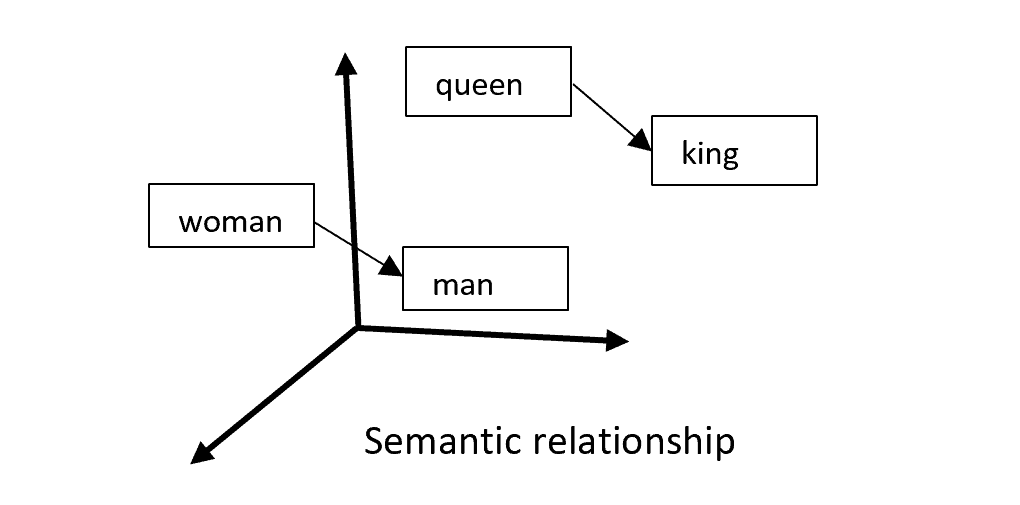
Word2vec starts with a simple observation: words which occur close together in a document are likely to share semantic similarities. For example, “king” and “queen” are likely to have similar meanings, be near each other in the document, and have related words such as “man” or “woman.” Word2vec takes this observation and applies it to a machine learning algorithm:

As a result, word2vec creates two types of vectors which represent each input word. These types are:

Word embedding or hidden representation (when the word is central)
Context word embedding or output representation (when the word is context)

We’ll describe below both types of word vectors in more detail.

3.1. Word Embedding

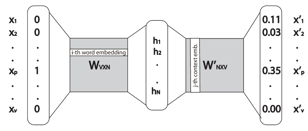
One way of creating a word2vec model is using the skip-gram neural network architecture. Briefly, this is a simple neural network with one hidden layer. It takes an input word as a one-hot vector, and outputs the probability vector from the softmax function with the same dimension as input.

Let’s define an input one-hot vector with $x_{V \times 1}$ . Then the hidden layer, $h_{1 \times N}$ , is a multiplication result between the transposed one-hot vector, $x_{V \times 1}$ , and weight matrix, $W_{V \times N}$ :

(1) $\begin{equation*} h = x^{T}W. \end{equation*}$

Since the vector $x$ is a one-hot vector, the hidden layer, or vector $h$ , will always be equal to the $i$ -th row of the matrix $W$ if the $i$ -th element in the vector $x$ is equal to 1. Here is an example:

(2) $\begin{equation*} [0, 0, 1, 0, 0] \cdot \begin{bmatrix} 4 &8 &16 \\ 17 &0 &11 \\ 2 &13 &4 \\ 9 &5 &4 \\ 28 &31 &19 \\ \end{bmatrix} = [2, 13, 4]. \end{equation*}$

Given the example, for a particular word $w$ , if we input its one-hot vector into the neural network, we’ll get the word embedding as a vector $h$ in the hidden layer. Also, we can conclude that the rows in the weight matrix $W$ represent word embeddings.

3.2. Context Word Embedding

After we compute the hidden layer, we multiply it with the second weight matrix $W`_{N \times V}$ . The output of this multiplication is the output vector $x'$ on which we use activation function softmax in order to get probability distribution:

(3) $\begin{equation*} x'=softmax(hW`). \end{equation*}$

Notice that the output vector has the same dimension as the input vector. Also, each element of that vector represents a probability that a particular word is in the same context as the input word.

From that, the context word embedding of the $i$ -th word is the $i$ -th column in the weight matrix $W`$ . The whole neural network can be seen in the image below:

4. Add, Concatenate, or Average Word Vectors

In order to understand what to do with both embedding vectors, we need to better understand weight matrices $W$ and $W'$ .

4.1. Relationship Between Two Embeddings

For example, lets take the word “cat” and observe its embeddings $cat_{we}$ and $cat_{ce}$ . If we calculate the dot product between two embeddings, we’ll get a probability that the word “cat” is located in its own context.

With the assumption that the context of a particular word is a few words before and after that word, which is usually the case, the probability that the word is located in its own context should be very low. Basically, it means that it’s very rare to have the same word twice, close one after another, in the same text.

From that, we can assume:

(4) $\begin{equation*} cat_{we} \cdot cat_{ce} = P("cat"|"cat") \approx 0. \end{equation*}$

Also, from the definition of the dot product, we have:

(5) $\begin{equation*} cat_{we} \cdot cat_{ce} = |cat_{we}||cat_{ce}| \cos{ \angle (cat_{we}, cat_{ce})}. \end{equation*}$

If we assume that the magnitude of any embedding is close to zero, then the same assumption will apply to every word in the vocabulary. It’ll indicate that the dot product between embeddings of all different words is close to zero, which is unlikely. Thus, we can assume that the cosine of the angle between embedding vectors is close to 0 or:

(6) $\begin{equation*} \cos{ \angle (cat_{we}, cat_{ce})} \approx 0 \end{equation*}$

This implies that the angle between two embedding vectors tends to $90^{\circ}$ or they’re orthogonal.

4.2. Add vs. Average

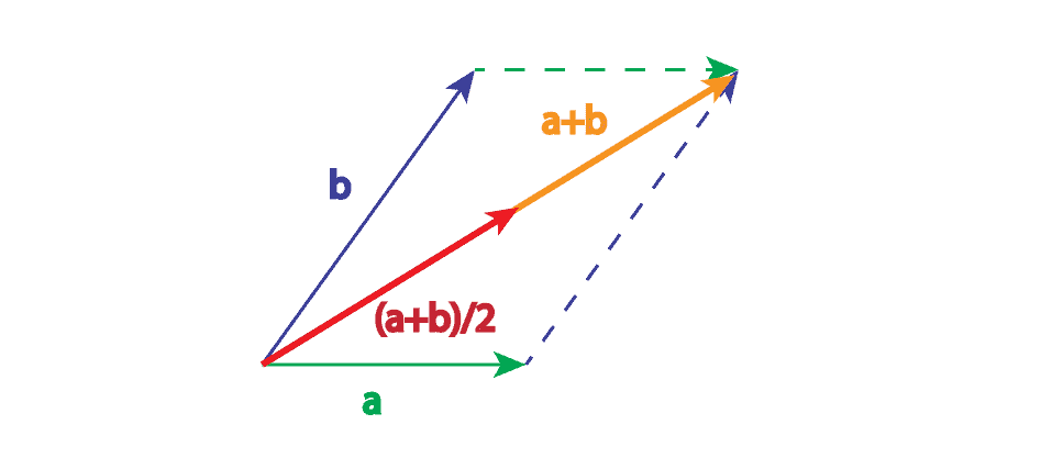
First of all, the visual representation of the sum of two vectors is a vector that we get if we place the tail of one vector to the head of another vector. The average of two vectors is the same vector, only multiplied by $\frac{1}{2}$ . From that perspective, there’s not much difference between the sum and average of two vectors, but the average vector has two times smaller magnitude. Thus, because of the smaller vector components, we can favor average over sum:

4.3. Combining Embedding Vectors

Let’s go back to the example with the word “cat” and its orthogonal vectors, $cat_{we}$ and $cat_{ce}$ . Let’s assume there’s a word “kitty” in the vocabulary. We’ll also assume that we have a perfect word2vec model which has learned that the words “cat” and “kitty” are synonyms, and they appear in a very similar context. This will mean that between word embeddings of those words, $cat_{we}$ and $kitty_{we}$ , is high cosine similarity.

Now let’s assume the perfect scenario where the cosine similarity is 1, and the angle between vectors is $0^{\circ}$ . We know that there’s a practice to use only word2vec word embeddings, while context embeddings are discarded. Furthermore, there’s no evidence that context vector will follow the same similarity as word embeddings. If we add the context embedding to the word embedding, we might get the following situation presented in the image below:

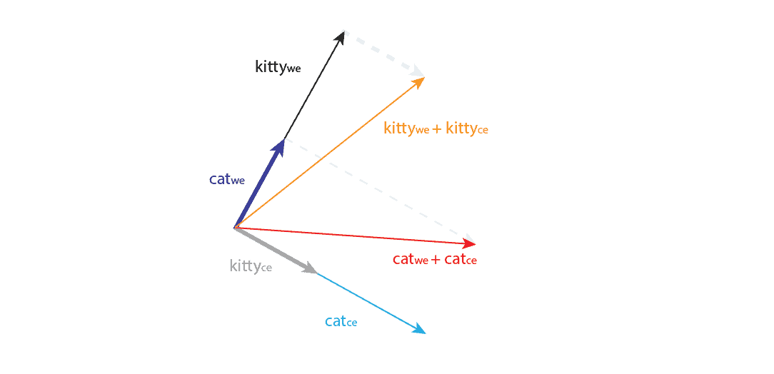
The angle between $cat_{we}$ and $kitty_{we}$ is $0^{\circ}$ , and these vectors are orthogonal to their corresponding context vectors. After addition, we see that the angle between sums is no longer $0^{\circ}$ .

Finally, it means that even with perfect conditions, the addition of the context vector to the embedding vector can disrupt the learned semantic representation in the embedding space. A similar conclusion can be made for a concatenation.

4.4. Experiments

Although it’s clear that the addition of context vectors will disrupt the learned semantic relationship of the embedding vectors, some experiments have been done using exactly this approach. It turned out that this operation can introduce additional knowledge into embedding space, and add a small boost in performance.

For instance, comparing human judgments of similarity and relatedness to cosine similarity between combinations of $W$ and $W'$ embeddings has shown that using only word embeddings, $W$ predicts better similarity while using one vector from $W$ and another from $W'$ gives better relatedness. For example, for the word “house,” using the first approach, most similar words were “mansion,” “farmhouse,” and “cottage,” while using the second approach, most related words were “barn,” “residence,” “estate,” and “kitchen.”

Moreover, the authors of the GloVe method used the sum of word and context embeddings in their work and achieved a small boost in performance.

5. Conclusion

Firstly, we need to make clear that the goal of this article is to discuss operations between vectors for one particular word, and not for combining word vectors from one sentence. How to get a vector representation for a sentence is explained in this article.

In this article, we explained in detail the logic behind the word2vec method and their vector in order to discuss the best solution for word vectors. Specifically, in the original word2vec paper, authors used only word embeddings as word vectors representation and discarded the context vectors.

In contrast, some experiments were done using different combinations of these vectors. As a result, it was found that the sum between these vectors can introduce additional knowledge, but doesn’t always provide a better result. Also, from geometrical interpretation, we know that the summer and averaged vectors will behave almost the same.

Furthermore, there’s no evidence for using concatenation operations between vectors. Finally, we recommend using only word embeddings, without context vectors, since this is a well-known practice and context vectors won’t give significantly better results. However, for research purposes, the sum or average might be worth exploring.

Full Archive

About Baeldung

Core Concepts

Operating Systems

Artificial Intelligence

Graph Theory

Latex