Finding Strongly Connected Components: Kosaraju’s Algorithm

1. Introduction

In this tutorial, we’ll discuss Kosaraju’s algorithm.

It’s one of the efficient algorithms for finding strongly connected components (SCCs) in directed graphs.

2. The Definition of Strongly Connected Components

Let’s assume we have a directed graph $G$ with $N$ vertices and $M$ edges. We’ll denote the vertices of $G$ by $G.V$ and the edges by $G.E$ .

The notion of SCC for directed graphs is similar to the notion of connected components for undirected graphs. Formally, SCC in $G$ is a subset of $G.V$ , such that:

Any two vertices in SCC are mutually reachable, i.e., for any two nodes $u, v$ in the same component, there’s a directed path from $u$ to $v$ and from $v$ to $u$
The addition of any vertex $x \notin$ SCC to SCC breaks the first condition

Any non-empty directed graph contains at least one SCC, and SCCs naturally divide $\boldsymbol{G.V}$ into non-intersecting subsets. Let’s check out some examples.

The graph below contains four SCCs – each vertex is a separate SCC:

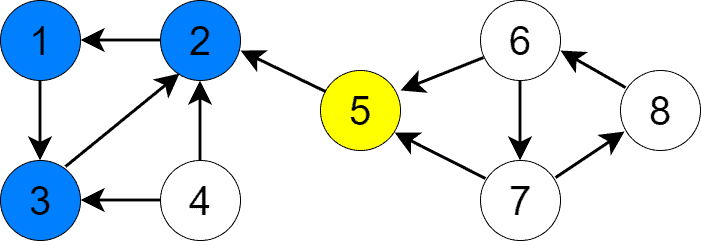
Below, we can see a bit more complex graph:

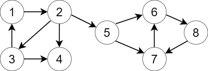
It also has four SCCs:

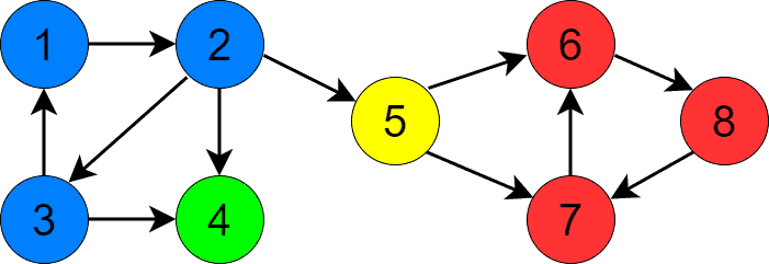
We’ve colored SCCs differently to distinguish them visually.

3. Kosaraju’s Algorithm

In this section, we’ll provide a step-by-step explanation of Kosaraju’s algorithm for finding SCCs. It has three steps.

3.1. Step 1

In the first step, we perform a DFS traversal to define the priorities of the vertices. More specifically, for each vertex, we remember when DFS finishes processing. The later DFS is done with a vertex, the higher its priority. This step is similar to topological sorting, but it’s not the same since the latter is only possible for DAGs.

The previous section shows the result of running this step for the graph. We started the process from vertex 1 (but we could start from any node). The priorities are red numbers:

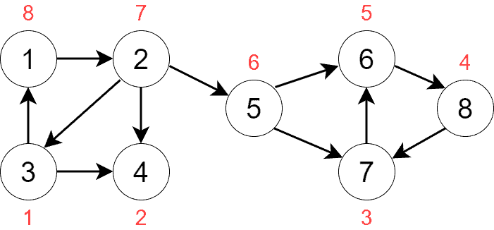
We push the vertices onto a stack during DFS traversal according to the priorities. The stack’s content at the end of the process will be: [3, 4, 7, 8, 6, 5, 2, 1].

3.2. Step 2

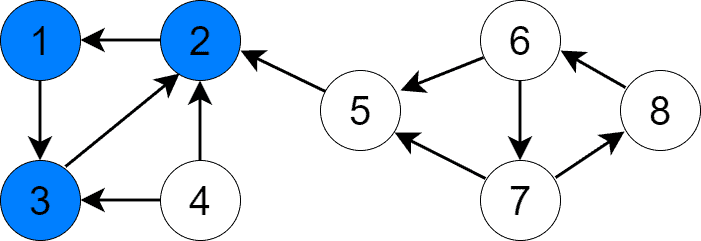
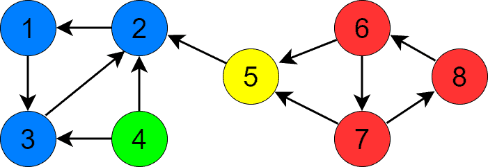
In the second step, we build the transpose graph of $G$ . The transpose graph is a graph that consists of the same vertices as the original graph, but the edge directions are reverted. Here’s the transpose graph $TG$ of $G$ :

We can construct $TG$ as a separate graph or invert the edges in $G.E$ .

3.3. Step 3

In the third step, we perform a DFS traversal on $\boldsymbol{TG}$ . Each DFS invocation finds one SCC. So, the number of SCCs is equal to the number of times we invoke DFS on $TG$ . Each time we call a DFS procedure, we use the non-visited node with the highest priority.

Let’s see how this step finds SCCs in our graph. After step 2, the highest-priority node is vertex 1, so we start the first DFS from that node. DFS visits vertices 1, 3, and 2 in this order and stops, finding us one SCC:

The next vertex with the highest priority is 5, as vertex 2 is already visited. We call DFS with node 5 as its argument and find the second SCC containing only that node:

Vertex 6 is the next vertex to visit. DFS visits 6, 7, and 8 in this order and returns:

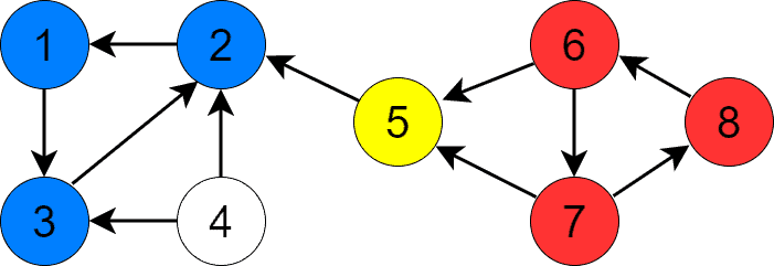
Lastly, we invoke DFS for vertex 4 and find the last SCC containing only that vertex:

At this point, we’ve found all the SCCs and the algorithm terminates.

4. The Pseudocode

First, let’s implement DFS. We need two of them: the common one traversing a graph and the second one building vertex priorities. Below we can find the pseudocode for the common DFS:

Below is the pseudocode for the DFS procedure, which builds vertex priorities:

Now, we’ll implement the logic of the transform graph creation:

4.1. The Pseudocode of Kosaraju’s Algorithm

All the pseudocodes are set up, it’s time to implement Kosaraju’s algorithm:

5. The Intuition Behind the Algorithm

Kosaraju’s algorithm correctly finds SCCs. But why? Let’s make some observations to improve the understanding of the algorithm.

5.1. The Properties of the Condensation Graph

The condensation graph $\boldsymbol{CG}$ of $\boldsymbol{G}$ is a graph that has SCCs of $\boldsymbol{G}$ as vertices. If $G$ contains edge $(v, u)$ , such that $v \in SCC1$ and $u \in SCC2$ , then $CG$ contains edge $(SCC1, SCC2)$ . $CG$ is a DAG because otherwise, it would contain a cycle and all SCCs in the cycle may have been merged into a single SCC. That contradicts the definition of SCC, according to which we can’t merge several SCCs to get a new bigger SCC. Below is the $CG$ of the graph from our previous examples:

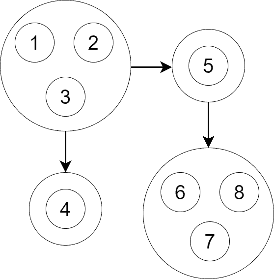
As we see, $CG$ is a DAG and it contains four vertices. Each vertice corresponds to an SCC.

5.2. Traversal Order

As $CG$ is a DAG, it’s possible to perform topological sorting on it. If SCC2 goes after SCC1 in topological sorting order, then step 1 of Kosaraju’s algorithm makes at least one vertex of SCC1 have a higher priority than all the vertices of SCC2. By doing so, it guarantees SCC1 is traversed before SCC2 in step 3.

5.3. The Properties of the Transpose Graph

The transpose graph $\boldsymbol{TG}$ has the same SCCs as the original graph $\boldsymbol{G}$ . Therefore, when we build $TG$ , semantically, only edges between SCCs are inverted. $TG$ also guarantees that when we start DFS in the highest priority vertex in step 3, DFS only visits the vertices in the SCC of that vertex. Inverting edges has the effect of isolating DFS from traversing outside of the current SCC. DFS can only visit the vertices in the current SCC and those of SCCs that have already been visited. DFS omits the latter.

6. The Complexity Analysis

We should use adjacency list representation for $\boldsymbol{G}$ in Kosaraju’s algorithm to have DFS run in $\boldsymbol{O(N + M)}$ time. The algorithm consists of three steps depending on the same variables $N$ and $M$ . So the algorithm’s complexity is the maximum of complexities of each step:

Step 1 is a DFS traversal of $G$ , which runs in $O(N + M)$
For transposing $G$ , we need to go over all the vertices and edges, so it’s another $O(N + M)$ operation
Step 3 is a DFS traversal of $TG$ , which also runs in $O(N + M)$

Thus, the overall complexity of Kosaraju’s algorithm is $\boldsymbol{O(N + M)}$ .

7. Conclusion

In this article, we covered Kosaraju’s algorithm. It’s a three-step algorithm for finding strongly connected components (SCCs).

Its first step is to run DFS to set the priorities of the vertices to their DFS exit times. Then, it builds the transpose of the original graph. Finally, the algorithm runs DFS on the transpose graph according to the vertex priorities defined in the first step. Each DFS invocation in the last step finds a separate SCC.

Full Archive

About Baeldung

Core Concepts

Operating Systems

Artificial Intelligence

Graph Theory

Latex