Interpolation and Regression: Similarities and Differences

1. Introduction

In this tutorial, we explain the concepts of interpolation and regression and their similarities and differences. Both words are frequently used in fields like banking, sports, literature, and law, among others. with different interpretations. Here, we’ll restrict the explanation to the point of view of Mathematics.

First, we’ll introduce both concepts in detail. Then, we’ll focus on their similarities and differences.

2. The Concept of Interpolation

Interpolation is a family of methods studied in Numerical Analysis (NA), a field of Mathematics. NA is oriented to finding approximate solutions to mathematical problems. Those solutions should be as accurate as possible.

Let’s assume that we have a set of points that correspond to a certain function. We don’t know the exact expression of the function, but just those points. And we want to calculate the value of the function on some other points. Interpolation allows for approximating this function by using other simpler functions. The approximated function should pass through all the points in the previously known set. Then, it could be used to estimate other points not included in the set.

2.1. Linear Interpolation

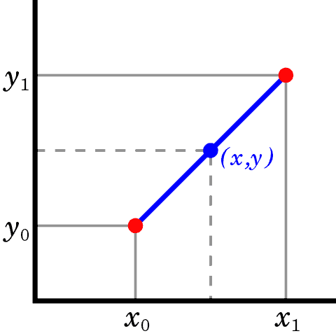
Linear interpolation is a method used to interpolate between two points by a straight line. Let’s consider two points ( $x_0$ , $y_0$ ), ( $x_1$ , $y_1$ ). Then the equation of the line passing by those points is y = a + bx, where:

$a = \frac{y_0.x_1 - y_1.x_0}{x_1 - x_0}$

$b = \frac{y_1 - y_0}{x_1 - x_0}$

In the following figure, the blue line represents the linear interpolant between the two red points.

Let’s assume that we’re approximating a value of some function f with a linear polynomial P. Then, the error R = f(x) – P(x) is calculated by:

$|R| < \frac{(x_1 - x_0)^2}{8}.max(f''(x))$

for x between the $x_0$ and $x_1$ .

We can also use linear interpolation with more than two points, but the error increases according to the degree of curvature of the function.

2.2. Polynomial Interpolation

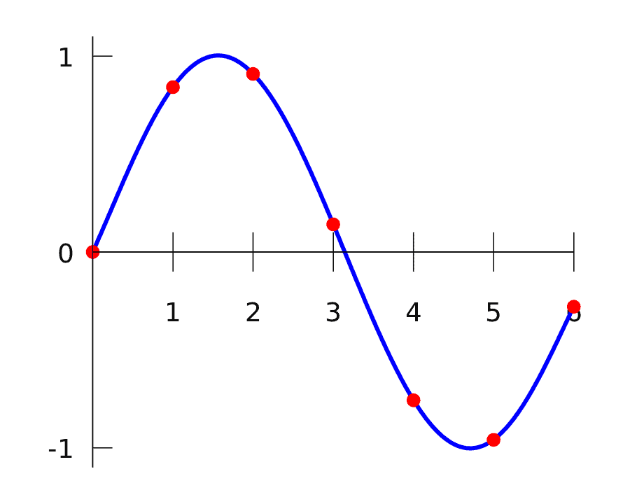
Polynomial interpolation is a method used to interpolate between $N$ points by a polynomial. Let’s consider a set with $N$ points. Then we can always find a polynomial that passes through those $N$ points. And this polynomial is unique. Polynomial interpolation is advantageous because polynomials are easier to evaluate, differentiate, and integrate.

There are different approaches to calculating the coefficients of the interpolation polynomial. One of them is using the Lagrange polynomial defined as:

$p(x) = \sum_{j=0}^{n}y_{j}.L_{n,j}(x)$

where:

$L_{n,j} = \prod_{k \ne j} \frac{x - x_k}{x_j - x_k}$

The following blue curve shows the interpolation polynomial adjusted to the red dots.

2.3. Spline Interpolation

Splines are special functions defined piecewise using low-degree polynomials. Spline’s popularity comes from its easy evaluation, accuracy, and ability to fit complex shapes. Polynomials used for splines are selected to fit smoothly together. The natural cubic spline is conformed by cubic polynomials. It is twice continuously differentiable. Moreover, its second derivative is zero at the endpoints.

Spline interpolation is smoother and more accurate than Lagrange polynomial and others. There are different formulae for calculating splines.

3. The Concept of Regression

Regression analysis is a family of methods in Statistics to determine relations in data. Those methods allow for evaluating the dependency of one variable on other variables. They are used to find trends in the analyzed data and quantify them. Regression analysis attempt to precisely predict the value of a dependent variable from the values of the independent variables. It also addresses measuring the degree of impact of each independent variable in the result.

The dependent variable is usually called the response or outcome. The independent variables are called features, and predictors, among others. This way, regression provides an equation to predict the response. For example, the value of the dependent variable is based on a particular combination of the feature values.

3.1. Linear Regression

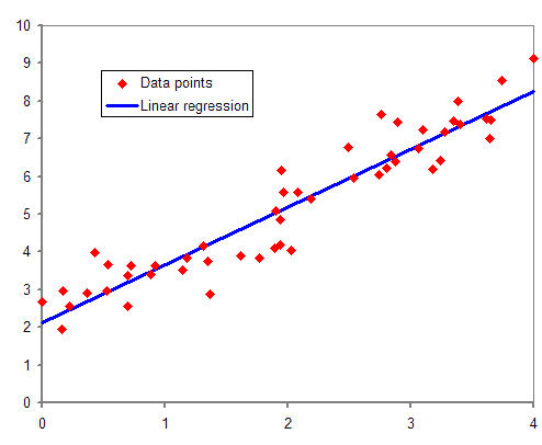
Linear regression approaches modeling the relationship between some dependent variables and other independent variables by a linear function. The linear regression model assumes a linear relationship between the dependent variable y and the independent variable x, like in the equation y = a + b.x, where y is the estimated dependent variable, a is a constant, and b is the regression coefficient, and x is the independent variable.

Linear regression considers that both variables are linearly related on average. Thus, for a fixed value of x, the actual value of y differs by a random amount from its expected value. Therefore, there is a random error ε, and the equation should be expressed as y = a + bx + ε, where ε is a random variable.

The actual values of a and b are unknown. Therefore, we need to estimate them from the sample data consisting of n observed pairs $(x_1, y_1), …, (x_n, y_n)$ :

Next, the blue line represents the regression model corresponding to the red points.

3.2. Least-Squares Method

The method of least squares allows estimating the values of a and b in the equation $y = a + b.x$ while minimizing the random error. Let’s assume that ε $_i = y_i$ – ŷ $_i$ for i = 1, …, n, where $y_i$ : the observed value, ŷ $_i$ is the estimated value and ε $_i$ is the residual between both values. The least-squares method minimizes the sum of the squared residuals between the observed and the estimated values.

The slope coefficient $b$ is calculated by:

$b = \frac{S_{xy}}{S_{xx}}$

where:

$S_{xy} = \sum(x_i.y_i) - \frac{(\sum x_i)(\sum y_i)}{n}$

$S_{xx} = \sum x_i^2 - \frac{(\sum x_i)^2}{n}$

The intercept a is calculated by:

$a = \frac{\sum y_i}{n} - b.\frac{\sum x_i}{n}$

4. Similarities and Differences Between Interpolation and Regression

Let’s look at the similarities and differences between interpolation and regression methods.

4.1. Similarities Between Interpolation and Regression

Interpolation and regression methods present similarities as they both:

Derive from Mathematics
Are oriented to process a set of data points
Are used to calculate new points
New calculated points should be accurate as possible
Model the dataset by a function
Have models for linear and non-linear cases

4.2. Differences Between Interpolation and Regression

Let’s review the main differences between the interpolation and regression methods:

Interpolation	Regression
Comes from Numerical Analysis	Comes from Statistics
Assumes that points in the dataset represent the values of a function accurately	Accepts inexact values
Assumes that one value of the independent variable just could be associated with one value of the dependent one	Accepts that the same value of the independent variable could have several values of the dependent variable associated
The approximated function should match exactly with all the dataset points	The approximated function does not have to match exactly with the dataset points
The error of the estimated values is bounded by some specific expression	The error of the estimated values is bounded on average
The approximated functions are frequently used for numerical integration and differentiation	The approximated functions are frequently used for prediction and forecasting

5. Conclusion

In this tutorial, we explained the concepts of interpolation and regression. We described their purpose and objectives. Some of the methods used in each field were explained. Finally, their similarities and differences were specified and described.

Learn Java Collections

Learn Spring

Learn Maven

View All Courses

Core Concepts

Operating Systems

Neural Networks

Graph Theory

Latex

Full Archive

About Baeldung