What Is the Difference Between Natural Cubic Spline, Hermite Spline, Bézier Spline and B-Spline?

1. Introduction

If we look at cars from the 1970s and the 1990s, there’s really one big difference in their designs. The ones from the ’70s are boxy, and the ones from the ’90s are curvy. Since then, cars have become curvier and curvier and aesthetically so appealing!

While the gasoline prices in the United States were low in the 60s, in Europe, fuel was always more expensive. In 1962, Pierre Bézier, an engineer at Renault, and Paul de Casteljau, a mathematician at Citroen, independently developed Bezier curves for fitting smooth curves and surfaces, allowing streamlined bodies and increased fuel efficiency.

In this tutorial, we’ll try to understand the mathematics underlying piecewise polynomial interpolation and explore some cool things we can do with these objects.

2. Thinking About Polynomials as Points or Vectors

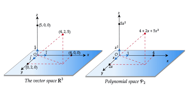
Polynomials are a basic means of approximation in all of science and mathematics. Let’s spend a moment reviewing our understanding of polynomials. A polynomial of degree $n$ is simply a function that takes real number $x$ as input and maps it to another real $y=p(x)$ , where $p(x)=a_nx^n + a_{n-1}x^{n-1}+\ldots+a_1x + a_0$ . However, polynomials in mathematics are special objects – they are vectors in the polynomial space $\mathcal{P}_n$ .

Let’s unpack this a bit. When we imagine vectors, we’ll see geometric arrows from our undergraduate physics lessons. And that’s totally cool!

We know that, any geometric vector $\vec{v}=(v_x,v_y,v_z)$ in $3$ -dimensional space can be written as a linear combination of the basis vectors $\hat{i}=(1,0,0)$ , $\hat{j}=(0,1,0)$ and $\hat{k}=(0,0,1)$ . The addition of two vectors is defined component-wise and the result is also a vector. Scalar multiplication is defined component-wise as, $c\vec{v} = cv_x \hat{i}+ cv_y \hat{j}+ cv_z \hat{k}$ .

Think about the collection of all polynomials of degree at most $2$ :

$\mathcal{P}_2 =\{a_2 x^2 + a_1 x + a_0 :a_j \in \mathbf{R} \text{ for }j=0,1,2\}$

Polynomials in the set $\mathcal{P}_2$ are isomorphic to geometric vectors in $3$ D-space. Any arbitrary degree $2$ polynomial can be expressed as a linear combination of the basis polynomials $1$ , $x$ and $x^2$ . These basis polynomials play the role of unit vectors:

Looking at it this way, the polynomial $p(x) = a_2 x^2 + a_1 x + a_0$ can be decomposed into three components: $a_2 x^2$ , $a_1 x$ and $a_0$ . From high-school math, we realize that, polynomials are also added component-wise.

What points or vectors are to $3$ D-space, polynomials are to the polynomial space $\mathcal{P}_2$ :

We can choose different basis vectors for $3$ -dimensional space. The vectors $(1,-2,1)$ , $(0,2,-2)$ and $(0,0,1)$ are also basis vectors for $3D$ -space. Pick any vector, such as $(4,2,5)$ . It can be expressed as a linear combination of the new basis vectors:

$\begin{pmatrix}4 \\ 2 \\ 5\end{pmatrix} = 4 \cdot \begin{pmatrix}1 \\ -2 \\ 1\end{pmatrix} + 5 \cdot \begin{pmatrix}0 \\ 2 \\ -2\end{pmatrix} + 11 \cdot \begin{pmatrix}0 \\ 0 \\ 1\end{pmatrix}$

This powerful idea also carries over to the set of polynomials $\mathcal{P}_2$ .

$1 - 2x+ x^2$ , $0 + 2x - 2x^2$ and $0 + 0x + x^2$ are another set of basis polynomials for $\mathcal{P}_2$ . Now, if we pick an arbitrary polynomial, such as $4 + 2x + 5x^2$ , it can be expressed as a linear combination, as follows:

$4 + 2x + 5x^2 = 4\cdot (1 - 2x + x^2) + 5 \cdot (0 + 2x - 2x^2) + 11(0 + 0x + x^2)$

3. The Case for Piecewise Polynomial Interpolation

Let’s review the problem of polynomial interpolation. We have an unknown underlying function or sometimes an expensive function $f$ . The values of the function $f$ are unknown on the interval $[a,b]$ , except for a finite subset of data-points:

$(x_0,y_0),(x_1,y_1),\ldots,(x_n,y_n)$

We’re interested to approximate the unknown or expensive function $f$ , by a polynomial $p$ .

From analytic geometry, we know that two points determine a straight line, and three points uniquely determine a parabolic curve of degree $2$ . In general, there is a unique interpolating polynomial $p(x)$ of degree $n$ that passes through $(n+1)$ data points.

In contrast, in piecewise polynomial interpolation, we construct a piecewise function consisting of multiple segments. The $j$ th segment, interpolates between the points $(x_{j-1},y_{j-1})$ and $(x_{j},y_{j})$ using the polynomial $p_j(x)$ .

3.1. Runge Phenomenon

Consider the approximation of the function $f(x) = 1/(1+25x^2)$ on $[-1,1]$ determined by interpolation on the equidistant grid with $m=11$ points:

$x_i = -1 + \frac{2(i-1)}{(m-1)}$

The graph of the degree- $10$ polynomial obtained from the equidistant grid – unlike the graph of $f$ , swings wildly between the grid points. The error from interpolation is large, especially near the endpoints, while near the center $[-\frac{1}{5},\frac{1}{5}]$ , it is fairly small. Such behavior is typical of equidistant interpolation. This is called the Runge phenomenon:

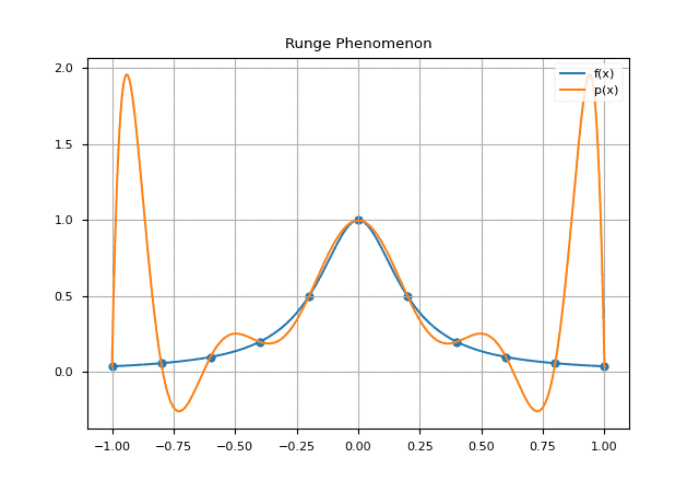
With piecewise polynomials, there is no need to fear equidistant data.

4. Bernstein Polynomials and Bézier Curves

Bézier curves are omniscient in computer graphics and computational geometry. A brief background of how these curves are built follows:

Consider a space-shuttle, that travels in a straight-line from a point $p_0=(x_0,y_0)$ to $p_1=(x_1,y_1)$ in time $t=1$ second. Let’s compute the position $p(t)=(x(t),y(t))$ of the space-craft at an arbitrary time $t$ . The point $p(t)$ divides the straight-line $p_0 p_1$ in the proportion $t:(1-t)$ , $t\in[0,1]$ . By the section formula, the coordinates of the point $p(t)$ are given by:

$\begin{align*} \left(x(t),y(t)\right) &= ((1-t)x_0 + tx_1,(1-t)y_0 + ty_1) \\ &= (1-t)(x_0,y_0) + t(x_1,y_1) \\ &= (1-t)p_0 + tp_1 \end{align*}$

This is the parametric equation of the motion of the space-craft. The points $p_0$ and $p_1$ control what the straight-line path looks like, so they are called control points.

Assume that, we have $3$ points $p_0$ , $p_1$ and $p_2$ . Imagine a blue particle $p_B$ moving from $p_0$ towards $p_1$ on a straight-line, a green particle $p_G$ moving from $p_1$ towards $p_2$ . Suppose, a third red particle $p_R$ moves along the straight-line joining blue and green particles:

How might we compute the trajectory of the red particle? By a double-application of the section formula, we have:

$\begin{align*} p_R(t) &= (1-t)\cdot p_B + t \cdot p_G \\ &= (1-t)((1-t)p_0 + tp_1) + t((1-t)p_1 + tp_2) \\ &= (1-t)^2 \cdot p_0 + 2t(1-t) \cdot p_1 + t^2 \cdot p_2 \end{align*}$

But, we saw earlier, that $(1-t)^2$ , $2t(1-t)$ and $t^2$ are like unit vectors. All quadratic curves can be generated by choosing different linear combinations of $(1-t)^2$ , $2t(1-t)$ and $t^2$ . Thus, the points $p_0$ , $p_1$ and $p_2$ control what the parabolic curve looks like.

The basis polynomials:

$\begin{align*} B_0(t) &= (1-t)^2 \\ B_1(t) &= 2t(1-t) \\ B_2(t) &= t^2 \end{align*}$

are called Bernstein basis polynomials. The quadratic curve corresponding to the control points $p_0$ , $p_1$ , $p_2$ is called the quadratic Bezier curve and is given by:

$p(t) = \sum_{i=0}^{2}p_i B_i(t)$

The quadratic Bezier curve interpolates between the points $p_0$ and $p_2$ , whereas $p_1$ is an off-curve point.

Computer graphics(CG) aficionados reserve the term control point for an off-curve point such as $p_1$ and refer to the on-curve points, as anchor points. In CG editors such as Adobe Illustrator, not all control points are known in advance. The shape of the quadratic curve is controlled by moving around the control points using the Pen tool (Bezier tool) until the curve has the desired shape. Thus, using the Bernstein basis to represent degree $2$ polynomials is advantageous. Moving $p_1$ has a direct and intuitive effect on the curve.

When rendering a TrueType font or a car body design, a smooth curve or surface is constructed, by chaining together several Bezier curves or patches.

5. Hermite Basis Polynomials and Cubic Hermite Interpolation

Hermite interpolation allows us to express any cubic polynomial in terms of two data-points $p(0)$ and $p(1)$ and the tangent slopes at these two points.

We derive the equation of a Hermite polynomial, by analyzing the physical motion of a particle under certain constraints. Let us imagine a particle that traverses a path given by the parametric equation $p(t) = at^3 + bt^2 + ct + d$ , where $t$ denotes time. The first derivative of this function is $p'(t) = 3at^2 + 2bt + c$ .

The position of the particle at times $t=0,1$ , $p(0)$ and $p(1)$ are known. The direction of motion of the particle at times $t=0,1$ , $p'(0)$ and $p'(1)$ are also known. We have:

$\begin{align*} p(0) &= d\\ p(1) &= a + b + c + d \\ p'(0) &=c \\ p'(1) &= 3a + 2b + c \end{align*}$

In the matrix form, we can write:

$\begin{bmatrix}p(0) \\ p(1) \\ p'(0) \\ p'(1)\end{bmatrix} = \begin{bmatrix}0 & 0 & 0 & 1 \\1 & 1 & 1 & 1 \\ 0 & 0 & 1 & 0 \\ 3 & 2 & 1 & 0 \end{bmatrix}\begin{bmatrix}a \\ b \\ c \\ d\end{bmatrix}$

Thus:

$\begin{align*} \begin{bmatrix}a \\ b \\ c \\ d\end{bmatrix} &= \left(\begin{bmatrix}0 & 0 & 0 & 1 \\1 & 1 & 1 & 1 \\ 0 & 0 & 1 & 0 \\ 3 & 2 & 1 & 0 \end{bmatrix}\right)^{-1}\begin{bmatrix}p(0) \\ p(1) \\ p'(0) \\ p'(1)\end{bmatrix}\\ &=\begin{bmatrix}2 & -2 & 1 & 1 \\-3 & 3 & -2 & -1 \\ 0 & 0 & 1 & 0 \\ 1 & 0 & 0 & 0 \end{bmatrix}\begin{bmatrix}p(0) \\ p(1) \\ p'(0) \\ p'(1)\end{bmatrix} \end{align*}$

Consequently:

$\begin{align*} \begin{bmatrix}t^3 & t^2 & t & 1 \end{bmatrix}\begin{bmatrix}a \\ b \\ c \\ d\end{bmatrix} &=\begin{bmatrix}t^3 & t^2 & t & 1 \end{bmatrix}\begin{bmatrix}2 & -2 & 1 & 1 \\-3 & 3 & -2 & -1 \\ 0 & 0 & 1 & 0 \\ 1 & 0 & 0 & 0 \end{bmatrix}\begin{bmatrix}p(0) \\ p(1) \\ p'(0) \\ p'(1)\end{bmatrix}\\ p(t) &= \begin{bmatrix}2t^3 - 3t^2 + 1 & -2t^3 + 3t^2 & t^3 - 2t^2 + t & t^3 - t^2 \end{bmatrix}\begin{bmatrix}p(0) \\ p(1) \\ p'(0) \\ p'(1)\end{bmatrix} \end{align*}$

In essence, we have managed to find the unique cubic curve determined by two data points $p(0)$ and $p(1)$ and the slopes at these points $p'(0)$ and $p'(1)$ .

6. Spline Functions

The most common piecewise polynomial interpolation uses spline functions. Mathematically, a spline $S(x)$ of degree $k$ , on a grid:

$\Delta = \{a = x_0 < x_1 < \ldots < x_{n} = b\}$

of data-points, also called knots, chains together $n$ sub-curves. Each sub-curve interpolates between two successive knot-points. Each sub-curve is a degree- $k$ polynomial:

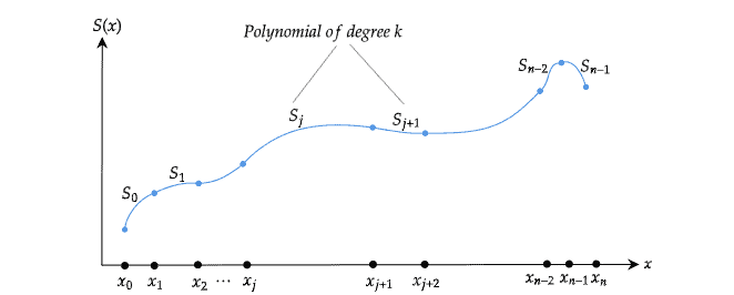
An additional requirement is that the whole spline $S(x)$ of degree- $k$ , must be $(k-1)$ times differentiable, and further its derivatives must be continuous. We discuss the consequences of this requirement, at length, further ahead.

We could use straight lines and parabolas for the segments of a spline. However, a polyline has sharp corners, so linear splines are not differentiable at the knot points. A quadratic curve has a constant second derivative. If we use quadratic curves, the curviness of one segment near a knot would not match the curviness of the preceding one. So, the most popular choice for the segments of a spline is cubic curves.

6.1. Cubic Spline Interpolant

A cubic spline uses cubic polynomials of degree $3$ to interpolate between successive knots. A cubic spline interpolant $S(x)$ satisfies the following conditions:

Each piece or segment $S_j(x)$ on the interval $[x_j,x_{j+1}]$ is a cubic polynomial.
$S_j(x_j) = y_j$ for each $j=0,1,\ldots,n-1$ .
$S_j(x_{j+1}) = S_{j+1}(x_{j+1})$ , $S_j'(x_{j+1}) = S_{j+1}'(x_{j+1})$ and $S_j''(x_j) = S_{j+1}''(x_{j+1})$ .

Condition (3) is simply a translation of the requirement that the whole spline should be $(k-1) = 2$ times differentiable and these derivatives must be continuous. As a crude approximation, we know that a continuous curve is one that can be drawn without lifting the pen from the paper. The individual segments of $S(x)$ are cubic polynomials, so they are continuous themselves. The only consideration is the continuity at the knot points.

For the curve to be continuous at any given knot-point $c$ , whether we approach it from the left, or we approach it from the right, the spline function $S(x)$ must approach $S(c)$ , regardless. Suppose the left piece is $S_j$ and the right piece is $S_{j+1}$ . This motivates $S_j(x_{j+1}) = S_{j+1}(x_{j+1})$ . A similar argument follows for the first and second derivatives because we would like those to be continuous.

6.2. Construction of the Cubic Spline

To construct the cubic spline interpolant on an interval that divided into $n$ subintervals, we require $n$ segments $S_0,S_1,\ldots,S_{n-1}$ . In line with condition (1), the segment $S_j(x)$ is a cubic polynomial of the form:

(1) $S_j(x) = a_j + b_j(x-x_j) + c_j(x-x_j)^2 + d_j(x-x_j)^3$

and has $4$ constants. Therefore, we have to determine the values of $4n$ constants.

The first and second derivatives of $S_j(x)$ are given by:

$\begin{align*} S_j'(x) &= b_j + 2c_j(x - x_j) + 3 d_j(x - x_j)^2 \\ S_j''(x) &= 2c_j + 6d_j(x - x_j) \end{align*}$

So, $S_{j+1}(x_{j+1}) = a_{j+1}$ , $S_{j+1}'(x_j) = b_{j+1}$ and $S_{j+1}''(x_{j+1}) = 2c_{j+1}$ . Also, the quantity $(x_{j+1} - x_j)$ appears often, so we let $h_j = (x_{j+1} - x_j)$ . Applying conditions (2) and (3), we obtain:

$\begin{align*} a_{j+1} = y_{j+1} &= a_j + b_jh_j + c_j h_j^2 + d_jh_j^3 && (2)\\ b_{j+1} &=b_j + 2c_j h_j +3d_jh_j^2 && (3)\\ c_{j+1} &= c_j + 3d_j h_j && (4) \end{align*}$

for each $j=0,\ldots,n-1$ . S0lving for $d_j$ in equation (4) and substituting this value in equations (2) and (3) gives, for each $j=0,1,\ldots,n-2$ , the new equations:

$\begin{align*} a_{j+1} &= a_j + b_jh_j + \frac{h_j^2}{3}(2c_j + c_{j+1}) && (5)\\ b_{j+1} &= b_j + (c_{j} + c_{j+1})h_j && (6) \end{align*}$

The final relationship is obtained by solving equation (5) first for $b_j$ :

(7) $b_j &= \frac{1}{h_j}(a_{j+1} - a_j) - \frac{h_j}{3}(2c_j + c_{j+1})$

and then with a reduction of the index, for $b_{j-1}$ . This gives:

(8) $b_{j-1} &= \frac{1}{h_{j-1}}(a_{j} - a_{j-1}) - \frac{h_{j-1}}{3}(2c_{j-1} + c_{j})$

Substituting these values into the equation derived from (6), with the index reduced by one, gives the linear system of equations:

(9) $\begin{align*} h_{j-1}c_{j-1} + 2(h_{j-1} + h_j)c_j + h_j c_{j+1} = \frac{3}{h_j}(a_{j+1} - a_{j}) - \frac{3}{h_{j-1}}(a_j - a_{j-1}) \end{align*}$

for each $j=1,2,\ldots,n-1$ . This system involves only the $\{c_j\}_{j=0}^{n}$ as unknowns. The values of $\{h_j\}_{j=0}^{n}$ and $\{a_j\}_{j=0}^{n}$ are given respectively by the spacing of the knots $\{x_j\}_{j=0}^{n}$ and the values $\{y_j\}_{j=0}^{n}$ at the knot-points. Once the values of $\{c_j\}_{j=0}^{n}$ are determined, it is a simple task to find the remainder of the constants $\{b_j\}_{j=0}^{n}$ and $\{d_j\}_{j=0}^{n}$ from equations (4) and (6).

6.3. The Natural Cubic Spline

An open question that arises from the preceding discussion is, whether a solution for the system of linear equations involving the unknowns $\{c_j\}_{j=0}^{n}$ exists, and if so, is it unique?

If we add two natural boundary conditions:

$\begin{align*} S''(a) &= 0 \\ S''(b) &= 0 \end{align*}$

then we get, $S_0''(x_0) = 2c_0 = 0$ and $S_{n-1}''(x_n) = 2c_n = 0$ . This results in a nice tridiagonal system of equations $Ax = b$ , that can be solved using Gaussian elimination:

$\begin{bmatrix} 1 & 0 & 0\\ h_0 & 2(h_0 + h_1) & h_2\\ & h_1 & 2(h_1+h_2) & h_3\\ \\ &&& h_{n-2} &2(h_{n-2} + h_{n-1})& h_{n-1} \\ &&& 0 & 0 & 1 \end{bmatrix}\begin{bmatrix} c_0\\ c_1 \\ c_2 \\ \vdots\\ c_{n-1}\\ c_n \end{bmatrix} = \begin{bmatrix} 0\\ \frac{3}{h_1}(a_2 - a_1) - \frac{3}{h_0}(a_1 - a_0) \\ \frac{3}{h_2}(a_3 - a_2) - \frac{3}{h_1}(a_2 - a_1) \\ \vdots\\ \frac{3}{h_{n-1}}(a_n - a_{n-1}) - \frac{3}{h_{n-2}}(a_{n-1} - a_{n-2}) \\ 0 \end{bmatrix}$

A quick numerical example should help crystallize these ideas. Suppose we’re given the data points $(0,0)$ , $(\pi/2,1)$ , $(\pi,0)$ and $(3\pi/2,-1)$ and $(2\pi,0)$ to form a cubic spline $S(x)$ to approximate the function $f(x) = \sin x$ . So, the matrix $A$ and the vectors $b$ and $x$ have the form:

$\begin{bmatrix} 1 & 0 & 0 & 0 & 0\\ \pi/2 & 2\pi & \pi/2 & 0 & 0\\ 0 & \pi/2 & 2\pi & \pi/2 & 0 \\ 0 & 0 & \pi/2 & 2\pi & \pi/2\\ 0 & 0 & 0 & 0 & 1 \end{bmatrix}\begin{bmatrix}c_0 \\ c_1 \\ c_2 \\ c_3 \\ c_4 \end{bmatrix} = \begin{bmatrix} 0 \\ -12/\pi \\ 0 \\ 12/\pi \\ 0 \end{bmatrix}$

The resulting cubic spline curve $S(x)$ is given by:

$S(x) = \begin{cases} 0.9549x - 0.1290 x^3 & x \in [0,\pi/2]\\ 1 - 0.6079x^2 + 0.129x^3 & x \in [\pi/2,\pi]\\ -0.9549x + 0.1290 x^3 & x \in [\pi,3\pi/2]\\ -1 + 0.6079x^2 - 0.1290x^3 & x \in [3\pi/2,2\pi] \end{cases}$

6.4. A Comparison of Different Piecewise Polynomial Interpolation Methods

Each interpolation method has its pros and cons.

A natural cubic spline segment assumes the position, the first derivative, and the second derivative from the preceding segment. Thus, the whole curve as well as its first two derivatives are continuous. However, any change in any segment changes the whole curve. Thus, the control is not local.

A B-Spline curve does not have to interpolate any of its control points. Unlike natural splines and Bezier curves, each segment is a weighted sum of only $d$ basis functions, where $d$ is the degree of the curve, giving the points local control. Thus, to create a large model with $C^2$ continuity and local control, we pretty much want to use cubic B-Splines.

The differences between various piecewise techniques is summarized below:

7. Applications

Today, spline functions are extensively used in the Computer-Aided Design (CAD) software for rendering car body surfaces. Complex surfaces can be modeled far beyond hand techniques.

Bezier curves have found use in computer graphics and typography. Cubic Bezier curves are the native curve format in Adobe Postscript fonts. Because, these curves are specified mathematically, they are infinitely scalable.

As with Bezier curves, a Bezier surface is defined by a mesh of control points.

As a small application, here is a rendition of the Utah Teapot in pastel color using Bezier surfaces:

The Utah Teapot is an icon of the computer graphics industry. It was one of the first computer graphics objects to be modeled using Bezier curves. The control points and Bezier patches of the Utah Teapot are publicly available.

8. Conclusion

In this article, we learnt, a few elementary methods of piecewise interpolation. Quadratic Bezier curves are parametrized by two data-points and one control-point. Cubic Hermite curves are parametrized by two end-points and the tangent slopes at the end-points.

A spline function $S(x)$ of degree $k$ on a grid of $(n+1)$ data points has $n$ segments, where each segment is a polynomial of degree $k$ , and its first $(k-1)$ derivatives are continuous. A natural cubic spline is a spline of degree $3$ , with the boundary condition that the spline is a straight-line near the first and last data points. It satisfies $S_0''(x_0) = S_{n-1}''(x_n) = 0$ .

Full Archive

About Baeldung

Core Concepts

Operating Systems

Artificial Intelligence

Graph Theory

Latex