Introduction to Curve Fitting | Baeldung on Computer Science

1. Overview

In this tutorial, we’ll briefly introduce curve fitting. First, we’ll present the basic terminology and the main categories of curve fitting, and then we’ll present the least-squares algorithm for curve fitting along with a detailed example.

2. Preliminaries

Let’s suppose that we are given a set of measured data points. Curve fitting is the process of finding a mathematical function in an analytic form that best fits this set of data. The first question that may arise is why do we need that. There are many cases that curve fitting can prove useful:

quantify a general trend of the measured data
remove noise from a function
extract meaningful parameters from the learning curve
summarize the relationships among two or more variables

3. Categories

Generally, curve fitting falls into two main categories based on how we handle the observed data:

3.1. Best Fit

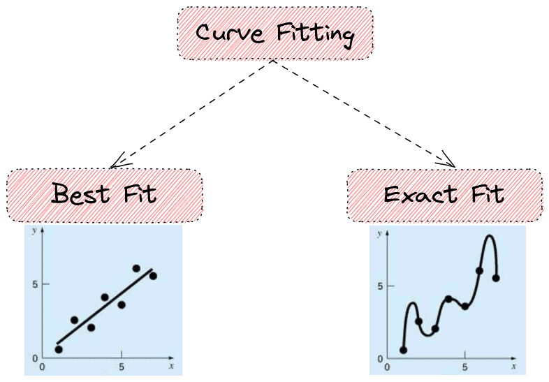
Here, we assume that the measured data points are noisy. So, we don’t want to fit a curve that intercepts every data point. Our goal is to learn a function that minimizes some predefined error on the given data points.

The simplest best fit method is linear regression, where the curve is a straight line. More formally, we have the parametric function $y = a x + b$ were $a$ is the slope and $b$ is the intercept and a set of samples $(x_1, y_1), (x_2, y_2), ..., (x_n, y_n)$ . Our goal is to learn the values of $a$ and $b$ to minimize an error criterion on the given samples.

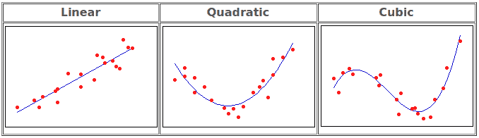
More generally, polynomial regression refers to the case that we want to fit a polynomial of a specific order $\mathbf{d}$ to our data:

linear when $d = 1: y = a x + b$
quadratic when $d = 2: y = a x^2 + b x + c$
cubic when $d = 3: y = a x^3 + b x^2 + c x + d$

In the functions above, we can observe that each time the parameters we want to learn are equal to $\mathbf{d+1}$ . Below, we can see some examples of curve fitting using different functions:

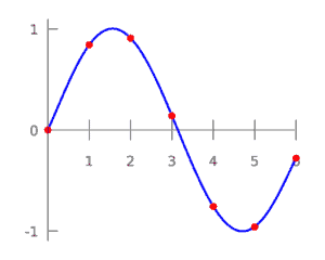
Also, we can fit any other function to our data like:

trigonometric functions
Gaussian functions
sigmoid functions

3.2. Exact Fit

In this case, we assume that the given samples are not noisy, and we want to learn a curve that passes through each point. It is useful in cases we want to derive finite-difference approximations or to find minimums, maximums, and zero crossings of a function.

In the figure below, we can see an example of an exact fit using polynomial interpolation.

4. Least-Squares Algorithm

There are many proposed algorithms for curve fitting. The most well-known method is least squares, where we search for a curve such that the sum of squares of the residuals is minimum. By saying residual, we refer to the difference between the observed sample and the estimation from the fitted curve. It can be used both for linear and non-linear relationships.

In the linear case when $d=1$ , the function we want to fit is $y = a x + b$ . So, we want to find the parameters $a, b$ so as to minimize $T = \sum_i (y_i - (b + a x_i))^2$ (sum of residuals).

In order to minimize the above term there are two conditions:

$\frac{\partial T}{\partial a} = 0 \to 2 \sum_i (y_i - (b + a x_i)) (-x_i) = 0 \to \sum_i x_i y_i = b \sum_i x_i + a \sum_i x_i^2$

$\frac{\partial T}{\partial b} = 0 \to 2 \sum_i (y_i - (b + a x_i)) = 0 \to \sum_i y_i = nb + a \sum_i x_i$

In non-linear least-squares problems, a very famous algorithm is the Gauss-Newton method. While we don’t have theoretical proof that the algorithm converges, it finds a proper solution in practice and is easy to implement.

5. Example

Here we’ll see an example of fitting a straight line in a set of samples using the least-squares method. Let’s suppose we have the following data:

$(1, 3), (2, 4), (3, 5), (4, 6), (5, 8)$

In the graph below, we can see the data in a scatter plot:

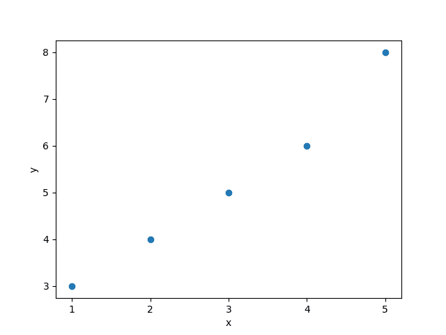
We want to fit the linear function $y = a x + b$ . If we replace our data in the equations we derived in the previous section we have the following results:

26 = 5b + 15a
90 = 15b + 55a

We solve the above system of two equations and two variables, and we find that $a=1.2$ and $b=1.6$ . So, we have the function $y = 1.2x + 1.6$ :

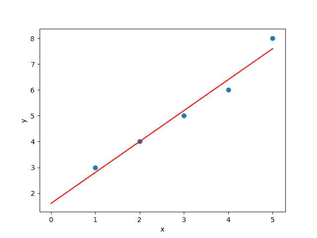
In the graph above, the red line corresponds to the fitted curve on the input data (blue dots). As we expected, the fitted line is the one that has the minimum distance from the input points.

6. Conclusion

In this tutorial, we talked about curve fitting. First, we made an introduction to the basic terminology and the categories of curve fitting. Then, we presented the least-squares algorithm both theoretically and through an example.

Full Archive

About Baeldung

Core Concepts

Operating Systems

Artificial Intelligence

Graph Theory

Latex