Basics of Polynomial Interpolation | Baeldung on Computer Science

1. Introduction

With the growth of data availability, strategies to process it becomes a big concern in the current computing scenario.

Nowadays, some technologies and computing paradigms, such as the Internet of Things (IoT) and big data, are particularly responsible for generating tons of data.

But, even obtaining lots of data, we may need to estimate extra data for specific purposes. Often, we have data in the XY format: for each X, there is a corresponding Y. Thus, in these scenarios, we can estimate an unknown Y for a new X in a given range through an interpolating polynomial.

Note that polynomial interpolation has several uses in computer science. Examples of such uses are data estimation (with some similarities with regression purposes) and screen resolution adaptions.

In this tutorial, we’ll learn basic concepts about polynomial interpolation. At first, we’ll see core concepts about polynomial interpolation. So, we’ll study a method for linear interpolation. Next, we’ll investigate a similar method to do quadratic interpolation. Finally, we’ll point out other interpolation methods.

2. Polynomial Interpolation

In many opportunities, we’ll have to analyze a lot of provided samples (XY data). However, we may not know the function that generated this data. So, if we need to analyze an intermediate value of X not provided, we’ll need to estimate its corresponding Y.

Preliminarily, it is relevant to highlight that, in our scenario, XY data consists of a pair of values. In specific, X is the input value that, after being processed, generates Y (the output value).

Polynomial interpolation enables us to determine a function that matches the XY data provided. It means that the function’s curve crosses points (X, Y) in the cartesian plane.

As the name suggests, polynomial interpolation generates a polynomial function. The general formula of a polynomial of degree $n$ is $f(x) = a_0 + a_1x + a_2x^2 + ... + a_nx^n$ .

Furthermore, we have a unique polynomial of degree $n$ matching $n+1$ samples of XY data. So, for instance, there is a single line crossing two particular points and a single parabola crossing three specific points.

Thus, our objective is to find these polynomials, using them to estimate Y for intermediate values of X (it means new X values between the minimal and maximum X used to interpolate the function).

2.1. An Abstract Example

Let’s consider that we have three samples in the format of XY data. X, in our example, indicates the time at which we collected the sample. Y, in turn, is the value measured when collecting the sample.

The following table shows our samples:

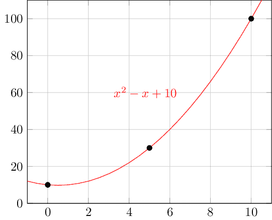
The following image presents our samples plotted in the cartesian plane:

And the image next shows the polynomial that interpolates our samples:

3. Linear Polynomial Interpolation

As the name suggests, linear interpolation aims to determine the linear function that embraces the provided XY data samples. Thus, the line generated by this function must cross the coordinate of XY data in the cartesian plane.

Functions describe lines in the cartesian plane when they are first-degree polynomials. In this way, we need two samples of XY data to execute a linear polynomial interpolation. So, lets consider the following generic samples: $(x1, y1)$ and $(x2, y2)$ .

To find the interpolating polynomial, first, we need to map our XY samples in the general formula of a first-degree polynomial function ( $y = a_0 + a_1 * x$ ). Doing that we’ll have $y1 = a_0 + a_1 * x1$ and $y2 = a_0 + a_1 * x2$ .

Since $x1$ , $x2$ , $y1$ , $y2$ are numeric values, we must only determine the coefficients $a_0$ and $a_1$ that satisfies the following system of equations:

There are different ways to solve a system of two equations: the substitution method, the comparison method, and the addition method. So, as any of these methods apply to the problem, we can choose the one that best fits it.

After solving the system of equations, we’ll have numeric values for both the coefficients $a_0$ and $a_1$ . Thus, we can finally replace the unknown coefficients from the general formula ( $y = a_0 + a_1 * x$ ) to determine our interpolating polynomial.

4. Quadratic Polynomial Interpolation

The quadratic interpolation has as final objective to find a quadratic function (second degree) that considers the XY samples. So, this function graphically describes a parabola that crosses all the provided samples.

As a second-degree equation, we’ll need to provide three XY samples to calculate the interpolating polynomial. In this way, let’s consider three generic numerical samples: (x1, y1), (x2, y2), and (x3, y3).

Similar to the linear interpolation, we’ll have to map the XY samples into the general formula of a second-degree polynomial function: $y = a_0 + a_1 * x + a_2 * x^2$ . Thus, mapping the samples, we’ll get three functions: $y1 = a_0 + a_1 * x1 + a_2 * x1^2$ , $y2 = a_0 + a_1 * x2 + a_2 * x2^2$ , and $y3 = a_0 + a_1 * x3 + a_2 * x3^2$ .

With the mapped functions, we can organize them into a system of three equations. In this manner, we can determine the coefficients a_0, a_1, and a_2 by solving the system:

Popular methods to solve systems of three equations are the elimination method and Crammer’s rule. Each method has different operations, advantages, and disadvantages. Thus, we should evaluate the problem to decide which one to use.

With the numerical values for the coefficients $a_0$ , $a_1$ , and $a_2$ , we can finally set them in the general formula of second-degree polynomial functions ( $y = a_0 + a_1 * x + a_2 * x^2$ ), thus creating our interpolating polynomial.

5. Other Polynomial Interpolation Methods

Besides the straightforward methods presented in the last sections, there are other methods to interpolate polynomials given a set of XY samples. Thus, in this section, we’ll have a brief presentation about these methods.

The first alternative method calls Lagrange Interpolating Polynomial. This method finds the lowest degree polynomial that interpolates a predetermined set of XY samples. So, let’s consider a set of XY samples $(x_1, y_1)$ , …, $(x_j, y_j)$ , … $(x_k, y_k)$ .

In this way, the general formula of the interpolating polynomial is $\sum^{k}_{j=0} y_j * l_j(x)$ . Where $l_j(x)$ is the Lagrange basis polynomial given by $l_j(x) = \prod_{m = 0, m \ne j}^{k} \frac{x - x_m}{x_j - x_m}$ .

Another alternative is called Newton’s Divided Difference Interpolation. This method process a set of XY samples $(x_1, y_1)$ , …, $(x_j, y_j)$ , … $(x_k, y_k)$ to find an interpolating polynomial by the divided differences technique.

For this method, first, we must determine all the divided differences for all possible combinations, from 2 samples to k samples of the provided set of XY samples: $f[x_1, x_2] = \frac{y_1 - y_0}{x_1 - x_0}$ , $f[x_1, x_2, x_3] = \frac{f[x_1, x_2] - f[x_2, x_3]}{x_2 - x_0}$ , and so on.

After that, we use the divided differences to find the interpolating polynomial through the following formula: $f(x) = f(x_0) + (x - x_0) * f[x_0, x_1] + (x - x_0) * (x - x_1) * f[x_0, x_1, x_2] + ... + (x - x_0) * (x - x_1) * ... * (x - x_k) * f[x_0, x_1, ..., x_k]$ .

6. Conclusion

In this tutorial, we learned about polynomial interpolation. First, we saw basic concepts of interpolation. Next, we examined a straightforward method to find a first-degree interpolating polynomial. In a similar way, we investigated a method for finding a second-degree interpolating polynomial. Finally, we outlined generic interpolation methods.

We can conclude that polynomial interpolation has several applications in computer science. But, as exist several methods to determine interpolating polynomials, we should analyze our particular problem, scenario, and resources to define which one to use.

Full Archive

About Baeldung

Core Concepts

Operating Systems

Artificial Intelligence

Graph Theory

Latex