Constructive Algorithms for Graph Colouring

1. Overview

In this tutorial, we’ll present well-known algorithms to solve the graph coloring problem. First, we’ll define the problem and give an example of it. After that, we’ll show the greedy, and DSatur approaches and discuss their optimality.

2. Defining the Problem

We’re given a graph consisting of vertices and edges connecting them. We’re asked to assign a colour to each vertex of the graph such that the following conditions are fulfilled:

1. No two adjacent vertices have the same colour. Remember that two vertices are considered adjacent if an edge connects them.
2. The number of colours used is the minimum possible.

For example, let’s consider the following graph:

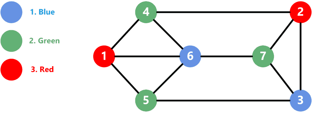
As we can see, the graph consists of vertices and edges connecting them. We numbered the vertices from 1 to 7 and the colours from 1 to 3. Overall, we used 3 colours to solve the problem. Note that no adjacent vertices have the same colour. Plus, our solution is the optimal one, as there’s no way to solve the problem using fewer colours.

Since the problem is considered NP-Complete, no efficient algorithm can solve all types of graphs. However, we’ll present two approaches that can give close to optimal solutions.

3. Greedy Approach

Let’s discuss the theoretical idea over an example and then jump into the implementation.

3.1. Theoretical Idea

In the greedy approach, we find a random ordering for the graph vertices. In addition, we number the colours starting from 1. Then, we iterate over the vertices individually and assign the feasible colour with the lowest number to each.

Let’s consider the same graph that we presented in section 2. Assume we use the following vertex ordering:

Then, we’ll get the following solution:

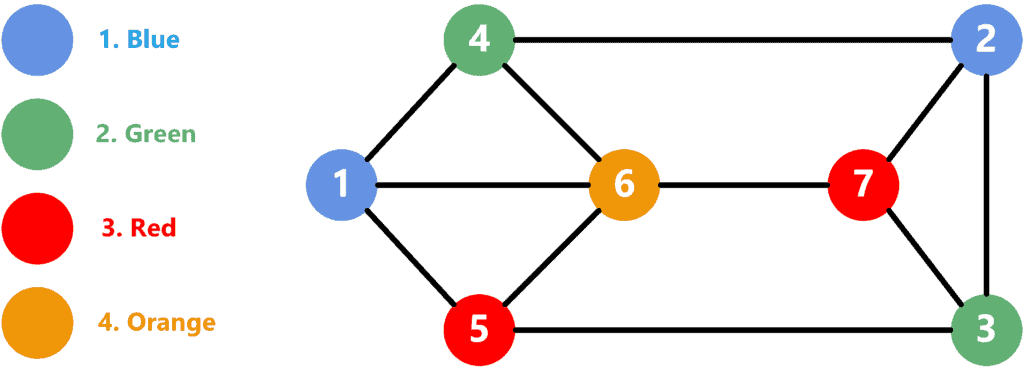
Solving the problem is done using the following steps:

1. Start with vertex 1 and use the first colour.
2. Vertex 2 doesn’t have any adjacent colours. Thus, we use the first one as well.
3. Vertex 3 has a blue vertex adjacent to it. Thus, we use the second one.
4. Similarly, vertex 4 has a blue vertex adjacent to it twice, so we also use the second one.
5. Vertex 5 has blue and green adjacent to it. Therefore, we have to use the third colour for it.
6. Vertex 6 now has blue, green, and red vertices adjacent to it. As a result, we have to use the new fourth colour.
7. Finally, vertex 7 has blue, green, and orange adjacents. Since the third colour (red) is not adjacent, we can use it.

As a result, we used 4 colours to solve the problem with this approach which is not optimal. However, it’s still close to the actual optimal result.

3.2. Implementation

Take a look at the implementation of the greedy approach:

We define a function that takes graph and the array of vertices in the order in which to apply the colouring. We start by defining an array called filled with zeros, indicating that we initially don’t have any colour assigned for the vertices.

Then, we iterate over all vertices. For each vertex, we iterate over all its edges and add the child’s colour to the set. After that, we move to find the correct colour to assign for the current vertex.

We start the with zero and perform multiple iterations to do that. In each iteration, we increase the by one and check if it’s not part of the . If so, we assign it to the current vertex.

Finally, we return the array containing the solution to our problem.

3.3. Time Complexity

Throughout the algorithm, we iterate over each node exactly once. We iterate over all its edges for each vertex and add the colours to a set. Thus, each edge is checked twice; once from each vertex, it connects. After that, we iterate over the colours to find the accepted one with the lowest number. Since each edge can make at most one colour invalid, we’ll perform steps before finding a valid solution for the vertex.

Therefore, assuming we use a HashSet with a constant complexity for adding elements, the overall time complexity will be .

4. DSatur Approach

Let’s discuss the theoretical idea first, then jump into the implementation.

4.1. Theoretical Idea

The DSatur name is short for Saturation Degree. This approach is similar to the greedy approach. However, it uses a more complex heuristic to determine the vertex order in which to apply the colouring. It uses the following criteria to choose the next vertex:

1. Choose the uncoloured vertex with the highest number of different adjacent colours. Therefore, it chooses the vertex with the highest saturation degree.
2. In case of a tie, choose the vertex with the highest degree. Remember that the degree of a vertex is the number of its edges.
3. If a tie still exists, choose the vertex randomly among the ones that satisfy the conditions.

Let’s consider the same graph as the one we presented in Section 2:

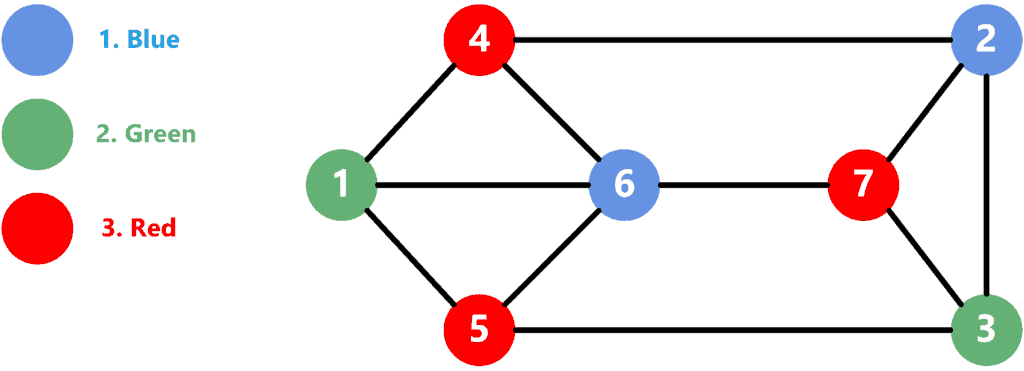
The solution was found with the following steps:

1. Since all vertexes are uncoloured yet, we choose the vertex with the highest degree. Thus, we choose vertex 6 and colour it with blue.
2. The vertices with the highest saturation degree are now {1, 4, 5, 7}. Since they all have a degree of 3, we choose vertex 1 randomly and use the second colour.
3. Now, vertices 4 and 5 have a saturation degree of two and an edge degree of three. We choose vertex 4 randomly and use the third colour for it.
4. Vertex 5 is the only vertex with a saturation degree of three. Therefore, we can use the third colour because blue and green are already adjacents.
5. All the remaining vertices have the same saturation degree of the same edge degree of 3, so we choose vertex 2 randomly. The only adjacent colour is the third one so we can use the first colour (blue).
6. Since all the vertices have the same saturation and edge degrees, we choose vertex 3 at random. Adjacent colours are the first and third ones. Thus, we can use the second colour (green).
7. The only vertex left is 7 and it has the first and second colours adjacent. Therefore, we choose the third colour for it (red).

Note that this approach generated a better solution than the greedy approach. In this case, it’s the optimal solution to use three colours. However, this algorithm is not guaranteed to give the optimal solution, but it usually gives a better one than the greedy approach.

In addition, the DSatur approach gives an optimal solution for bipartite graphs. This is because no matter which vertex we start from, we always choose the one with the highest saturation degree. Since bipartite graphs don’t have edges among edges of the same side, the next chosen vertex will be on the other side and assigned a different colour. This process will continue until we find a solution for all the vertices.

4.2. Implementation

Take a look at the implementation of the algorithm:

We define a function called which takes the graph and vertices as inputs. Similarly to the greedy approach, we define the array that will hold the colour of each vertex. In addition, we define the array, which holds the set of adjacent colours for each vertex, and the priority queue , which holds the vertices sorted by their saturation degree (initially zero) and the edge degree.

Next, we perform multiple steps. We extract a node from the queue in each step and get its vertex. If the vertex is already coloured, we have popped a node with the same vertex but with a higher saturation degree.

If the vertex is not coloured yet, we find a solution for it using the same approach as the greedy approach. After that, we iterate over all the children of the current node, update their saturation and push a new node to the queue with the child and the new saturation. Note that even if we push a node for the same vertex, it will be with lower saturation. Thus, it will be pulled after this node and just ignored.

Finally, we return the array, which holds the answer for each vertex.

4.3. Time Complexity

The algorithm performs multiple steps until the queue is empty. However, the number of steps can’t exceed the number of edges because each edge adds at most one new node to the queue. In addition, after we pop the nodes from the queue, we only process each vertex once. In this process, we iterate over all the children of the node. Thus, overall, we only iterate over the total number of edges.

Note that we perform multiple steps until we find a suitable colour for the vertex. However, these steps won’t exceed the number of edges as we described in the greedy approach. The only added complexity is with adding new nodes to the priority queue.

Given the above facts, the overall complexity is .

5. Comparison

The greedy approach has a lower time complexity than the DSatur approach. Thus, it can be preferred in cases where time complexity is a very critical factor. Nevertheless, the DSatur approach has a better chance of finding a more optimal solution than the greedy approach. Plus, the time complexity is only slightly higher than the greedy approach.

Therefore, we prefer to use the DSatur approach over the greedy approach.

6. Conclusion

In this tutorial, we covered some constructive algorithms for graph colouring. We defined the problem and explained it with an example. Then, we defined two approaches to solve the problem. We discussed the theoretical idea, the implementation, and the time complexity for each of them. We summarized with a comparison between both approaches and when to use each.