How to Find If a Graph Is Bipartite? | Baeldung on Computer Science

1. Overview

In graph theory, a bipartite graph is a special kind of graph that consists of two vertex sets. In this tutorial, we’ll discuss a general definition. We’ll also present an algorithm to determine whether a given graph is bipartite or not.

2. Bipartite Graph Definition

Let’s consider a graph $G(V, E)$ . The graph $G$ is a bipartite graph if:

The vertex set $V$ of $G$ can be partitioned into two disjoint and independent sets $V_1$ and $V_2$
All the edges from the edge set $E$ have one endpoint vertex from the set $V_1$ and another endpoint vertex from the set $V_2$

Let’s try to simplify it further. Now in graph $G$ , we’ve two partitioned vertex sets $V_1$ and $V_2$ . Suppose we’ve an edge $(E_1, E_2) \in E$ . Now according to the definition of a bipartite graph, the edge $(E_1, E_2)$ should connect to one vertex from set $V_1$ and another from set $V_2$ .

3. An Example

It’s now time to see an example of a bipartite graph:

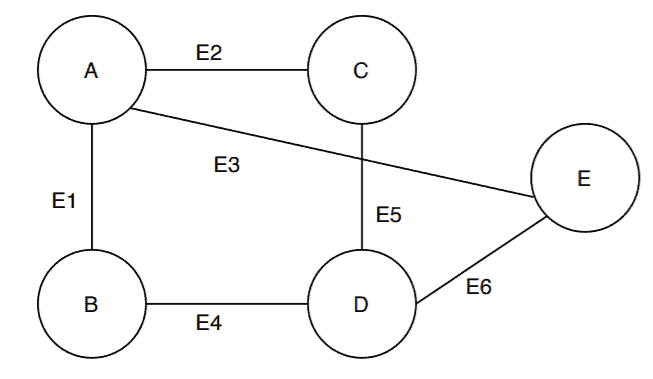
Here, we’ve taken a random graph $G_1(V, E)$ . Now, to satisfy the definition of a bipartite graph, the vertex set needs to be partitioned into two sets such that each edge joins the two vertex sets.

Is it possible to partition the vertex set of $G_1$ so that it satisfies the bipartite graph definition? Let’s find out:

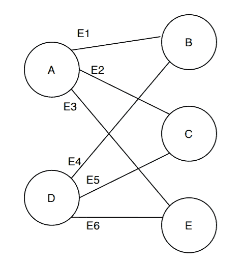
This is the same graph $G_1$ , just with a different representation. Here, we partition the vertex set $V=(A, B, C, D, E)$ into two disjoint vertex sets $V_1 = (A, D)$ and $V_2 = (B, C, E)$ .

Also, we can see the edges from the edge set $E = (E_1, E_2, E_3, E_4, E_5, E_6)$ follows the definition of a bipartite graph. Each edge has one endpoint in $V_1$ and another endpoint in $V_2$ . There are no edges whose both endpoints belong to $V_1$ or $V_2$ .

Therefore, we can conclude that the graph $G_1$ is a bipartite graph.

4. Properties

Bipartite graphs have some very interesting properties. In this section, we’ll discuss some important properties of a bipartite graph.

If a graph is a bipartite graph then it’ll never contain odd cycles.

In graph $G_1$ , a random cycle would be $ABDCA$ . Another one is $DEACD$ .

The length of the cycle is defined as the number of distinct vertices it contains. In both of the above cycles, the number of vertices is $4$ . Hence these are even cycles.

The subgraphs of a bipartite graph are also bipartite.

In graph $G_1$ , let’s select a random subgraph $G_S(V_S, E_S)$ . Here $V_S = (A, B, C, D)$ and $E_S = (E_1, E_2, E_4, E_5)$ . This subgrah $G_S$ of $G$ is also a bipartite graph.

A bipartite graph is always 2-colorable, and vice-versa.

In graph coloring problems, 2-colorable denotes that we can color all the vertices of a graph using $2$ different colors such that no two adjacent vertices have the same color.

In the case of the bipartite graph $G_1$ , we have two vertex sets and each edge has one endpoint in each of the vertex sets. Therefore, all the vertices can be colored using $2$ different colors and no two adjacent nodes will have the same color.

In an undirected bipartite graph, the degree of each vertex partition set is always equal.

In the example graph $G_1$ , the partitions are: $V_1 = (A, D)$ and $V_2 = (B, C, E)$ . Now the sum of degrees of vertices $A$ and $D$ will be the degree of the set $V_1$ . $A$ and $D$ both are of degree $3$ . Hence, the degree of $V_1$ is $6$ .

The degree of $V_2$ is the sum of degrees of vertices $B$ , $C$ , and $E$ . The vertices $B$ , $C$ , and $D$ are of degree $2$ each. Hence, the degree of the set $V_2$ is $6$ . So as $G_1$ is a bipartite graph, the degree of the two vertex partition sets are of equal degree.

5. Algorithm

In this section, we’ll present an algorithm that will determine whether a given graph is a bipartite graph or not.

algorithm IsBipartite(G(V, E), S):
    // INPUT
    //     G(V, E) = a graph with vertices V and edges E
    //     S = starting vertex
    // OUTPUT
    //     Flag indicating if if the graph is bipartite

    r <- create an empty queue
    color[S] <- RED
    r.enqueue(S)

    while r is not empty:
        n1 <- r.dequeue()
        for each n2 in n1.Adj():
            if color[n2] = null:
                if color[n1] = RED:
                    color[n2] = BLUE
                else:
                    color[n2] = RED
                r.enqueue(n2)
            else:
                if color[n2] = color[n1]:
                    return 'Graph is not Bipartite'

    return 'Graph is Bipartite'

This algorithm uses the concept of graph coloring and BFS to determine a given graph is bipartite or not.

This algorithm takes the graph $G(V, E)$ and a starting vertex $S$ as input. The algorithm returns either the input graph $G$ is bipartite or the graph is not a bipartite graph.

The steps of this algorithm are:

Assign a red color to the starting vertex $S$
Find the neighbors of the starting vertex and assign a blue color
Find the neighbor’s neighbor and assign a red color
Continue this process until all the vertices in the graph are assigned a color
During this process, if a neighbor vertex and the current vertex have the same color then the algorithm terminates. The algorithm returns that the graph is not a bipartite graph

We’ve used a queue data structure $r$ to store and manage all the neighbor vertices.

6. Running the Algorithm on a Graph

In this section, we’ll run the algorithm on a sample graph to verify that the algorithm gives the correct output:

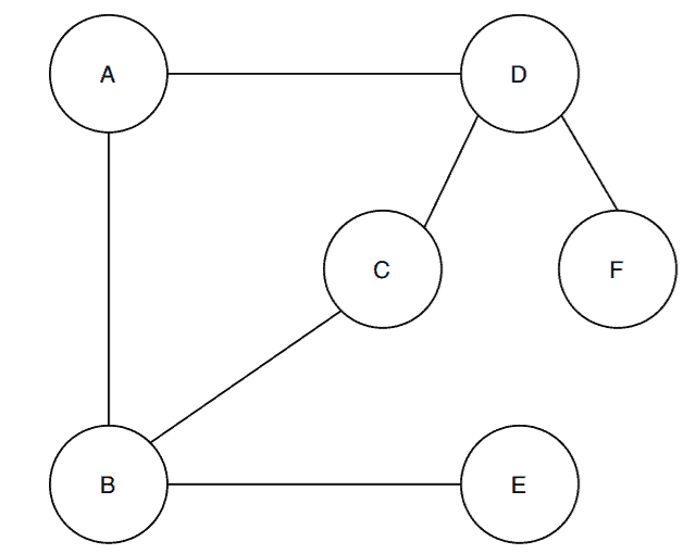
We’ve taken a sample graph $G_2$ and vertex set $V = (A, B, C, D, E, F)$ has $6$ vertices. Here we’re picking the vertex $A$ as the starting vertex. So let’s start the first step:

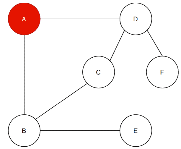
So the first step of the algorithm is to fill the starting vertex with the red color. The next step is to find the neighbor vertices of the vertex $A$ and fill them with the color blue:

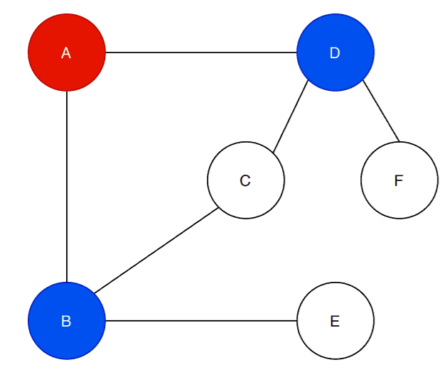
The vertex $A$ has two adjacent vertices: $B$ and $D$ . The algorithm first checks if the adjacent vertices are already filled with color. In our case, they are not filled. The algorithms fill the vertex $B$ and $D$ with the blue color.

We then choose any of the newly filled vertices and find the neighbors. Let’s choose the vertex $B$ :

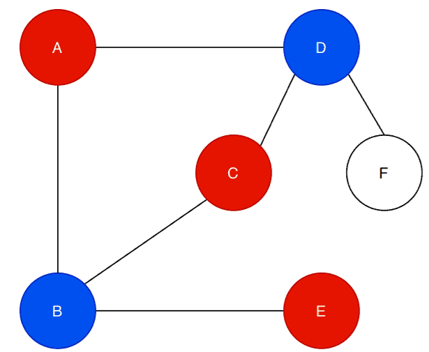
In graph $G_2$ , the vertex $B$ is adjacent to vertex $C$ and $E$ . Now the algorithm first checks if the vertices are already filled with some color. In our case, the vertices are not filled with color.

Next, the algorithm checks the color of the vertex $B$ . As the color of $B$ is blue, so the algorithm fills $C$ and $E$ with red:

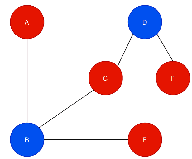
Now, the algorithm checks the adjacent vertices for the $D$ . The vertex $D$ has two adjacent vertices: $C$ and $F$ . Again, the algorithm checks whether the vertices already filled with color or not. In this case, the vertex $C$ is already filled with color. But the vertex $F$ is not filled yet.

The algorithm checks the color of the vertex $D$ . As the vertex $D$ is filled with the blue color, the algorithm fills the vertex $F$ with the red color. The algorithm continues this process until it checks all the vertices and it’s neighbors once.

Now, we can see that in the graph $G_1$ , no adjacent vertices have the same color. Also, we can see two clear partitions of the vertex set: $V_1 = (B, D)$ and $V_2 = (A, C, E, F)$ .

Therefore, the algorithm returns that the graph $G_2$ is a bipartite graph.

7. Time Complexity Analysis

In the algorithm, first, we traverse each vertex once. Then for each vertex, we visit each neighbor of a vertex once. The algorithm uses BFS for traversing. BFS takes $\mathcal{O}(V + E)$ time.

For storing the vertices, we can either use an adjacency matrix or an adjacency list.

Now if we use an adjacency matrix, then it takes $\mathcal{O}(V ^2)$ to traverse the vertices in the graph. So, if we use an adjacency matrix, the overall time complexity of the algorithm would be $\mathcal{O}(V ^2)$ .

On the other hand, an adjacency list takes $\mathcal{O}(V + E)$ time to traverse all the vertices and their neighbors in the graph. Therefore, if we use an adjacency list in the algorithm then the overall time complexity will be $\mathcal{O}(V + E)$ .

8. Conclusion

In this tutorial, we’ve discussed the bipartite graph in detail.

We’ve presented a graph coloring based BFS algorithm to determine if a graph is bipartite or not.

Finally, we’ve analyzed the time complexity of the given algorithm.

Full Archive

About Baeldung

Core Concepts

Operating Systems

Artificial Intelligence

Graph Theory

Latex