Gradient Boosting Trees vs. Random Forests | Baeldung on Computer Science

1. Introduction

In this tutorial, we’ll cover the differences between gradient boosting trees and random forests. Both models represent ensembles of decision trees but differ in the training process and how they combine the individual tree’s outputs.

So, let’s start with a brief description of decision trees.

2. Decision Trees

A decision tree is a tree-shaped plan of checks we perform on the features of an object before making a prediction. For example, here’s a tree for predicting if the day is good for playing outside:

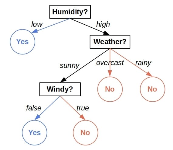
Each internal node inspects a feature and directs us to one of its sub-trees depending on the feature’s value and the leaves output decisions. Every leaf contains the subset of training objects that pass the checks on the path from the root to the leaf. Upon visiting it, we output the majority class or the average value of the leaf’s set.

However, trees are unstable. Slight changes to the training set, such as the omission of a handful of instances, can result in totally different trees after fitting. Further, trees can be inaccurate and perform worse than other machine-learning models on many datasets.

The ensembles of trees address both issues.

3. Random Forests

A random forest is a collection of trees, all of which are trained independently and on different subsets of instances and features. The rationale is that although a single tree may be inaccurate, the collective decisions of a bunch of trees are likely to be right most of the time.

For example, let’s imagine that our training set $\mathcal{D}$ consists of $200$ instances with four features: $A$ , $B$ , $C$ , and $D$ . To train a tree, we randomly draw a sample $\mathcal{S}$ of instances from $\mathcal{D}$ . Then, we randomly draw a sample of features. For instance, $A$ and $C$ . Once we do that, we fit a tree to $\mathcal{S}$ using only those two features. After that, we repeat the process choosing different samples of data and features each time until we train the desired number of trees.

3.1. Advantages and Disadvantages

Forests are more robust and typically more accurate than a single tree. But, they’re harder to interpret since each classification decision or regression output has not one but multiple decision paths. Also, training a group of $m$ trees will take $m$ times longer than fitting only one. However, we can train the trees in parallel since they are by construction mutually independent.

4. Gradient Boosting Trees

Gradient boosting is a widely used technique in machine learning. Applied to decision trees, it also creates ensembles. However, the core difference between the classical forests lies in the training process of gradient boosting trees. Let’s illustrate it with a regression example (the $x_i$ are the training instances, whose features we omit for brevity):

$\begin{matrix} x & y \\ \hline x_1 & 10 \\ x_2 & 11 \\ x_3 & 13 \\ x_4 & 20 \\ x_5 & 22 \\ \end{matrix}$

The goal is to train multiple trees one stage at a time. In each, we construct a single tree to correct the errors of the previously fitted ones.

4.1. Training the Gradient Boosting Trees: the First Tree

First, we train a decision tree ( $f_1$ ) using all the data and features. Then, we calculate its predictions $f_1(\cdot)$ and compare them to the ground truth $y$ :

$\begin{matrix} x & y & f_1(x) & y - f_1(x) \\ \hline x_1 & 10 & 9 & 1\\ x_2 & 11 & 13 & -2\\ x_3 & 13 & 15 & -2\\ x_4 & 20 & 25 & -5\\ x_5 & 22 & 31 & -9\\ \end{matrix}$

4.2. The Second Tree

As we see, the first tree seems off. How can we improve it? Well, an intuitive strategy is to fit another regressor $\boldsymbol{f_2}$ on the residuals $\boldsymbol{y - f(1)}$ . If it’s accurate, then $f_1(x) + f_2(x) \approx f_1(x) + y - f_1(x) = y$ , and we’ll get a precise model. To evaluate the adequacy of $f_1 + f_2$ , we calculate the new residuals $y - f_1(x) - f_2(x)$ :

$\begin{matrix} x & y & f_1(x) & f_2(x) & y - f_1(x) - f_2(x)\\ \hline x_1 & 10 & 9 & 0.5 & 0.5\\ x_2 & 11 & 13 & 1 & -3\\ x_3 & 13 & 15 & -1 & -1\\ x_4 & 20 & 25 & -2 & -3\\ x_5 & 22 & 31 & -4 & -5\\ \end{matrix}$

If we’re satisfied, we stop here and use the sequence of trees $f_1$ and $f_2$ as our model. However, if the residuals $y - f_1(x) - f_2(x)$ indicate that the sequence $f_1 + f_2$ has a too high error, we fit another tree $f_3$ to predict $y - f_1(x) - f_2(x)$ and use the sequence $f_1 + f_2 + f_3$ as our model.

We repeat the process until we reduce the errors to an acceptable level or fit the maximum number of trees.

4.3. Advantages and Disadvantages

Gradient boosting trees can be more accurate than random forests. Because we train them to correct each other’s errors, they’re capable of capturing complex patterns in the data. However, if the data are noisy, the boosted trees may overfit and start modeling the noise.

4.4. The Main Differences with Random Forests

There are two main differences between the gradient boosting trees and the random forests. We train the former sequentially, one tree at a time, each to correct the errors of the previous ones. In contrast, we construct the trees in a random forest independently. Because of this, we can train a forest in parallel but not the gradient-boosting trees.

The other principal difference is in how they output decisions. Since the trees in a random forest are independent, they can determine their outputs in any order. Then, we aggregate the individual predictions into a collective one: the majority class in classification problems or the average value in regression. On the other hand, the gradient boosting trees run in a fixed order, and that sequence cannot change. For that reason, they admit only sequential evaluation.

4.5. But Where Are Gradients in All This?

We haven’t mentioned gradients until now, so why do we refer to these trees as gradient boosting trees?

Let’s assume we use the square loss to measure the error of a regression model $f$ on the data $\left\{ (x_i, y_i) \right\}_{i=1}^{n}$ . Then, our goal is to minimize:

$J = \frac{1}{2} \sum_{i=1}^{n} (y_i - f(x_i))^2$

The partial derivative $\frac{\partial J}{\partial f(x_i)}$ is:

$\frac{\partial J}{\partial f(x_i)} = \frac{1}{2}\cdot 2(y_i - f(x_i)) \cdot (-1) = f(x_i) - y_i$

It’s equal to the negative residual and tells us how to change each $f(x_i)$ to minimize $J$ . But that’s how Gradient Descent works! To minimize $J$ with respect to $f(x_i)$ , we update each $f(x_i)$ by subtracting the weighted derivative:

$f(x_i) \leftarrow f(x_i) -\rho \cdot \frac{\partial J}{ \partial f(x_i)} \qquad (\rho = \text{ the learning rate})$

By training the tree $\boldsymbol{f_2}$ to approximate the negative residuals of $\boldsymbol{f_1}$ and correcting $\boldsymbol{f_1}$ by replacing it with $\boldsymbol{f_1 + f_2}$ , we perform a gradient update step in the Gradient Descent algorithm. Each new tree corresponds to another step of Gradient Descent.

The vector of negative residuals of $f$ isn’t necessarily equal to the $f$ ‘s gradient. They will differ if we use other loss functions. So, instead of to residuals, we fit the trees $\boldsymbol{f_2, f_3, \ldots}$ to the negative gradients of $\boldsymbol{f_1, f_1 + f_2, \ldots}$ , respectively. That’s why such trees are known as gradient boosting trees.

5. Conclusion

In this article, we presented the gradient-boosting trees and compared them to random forests. While both are ensemble models, they build on different ideas. We can fit and run the former ones only sequentially, whereas the trees in a random forest allow for parallel training and execution.

Full Archive

About Baeldung

Core Concepts

Operating Systems

Artificial Intelligence

Graph Theory

Latex