

Yes, we're now running our only Summer Sale. All Courses are 30% off until 20th July, 2026:
Learn through the super-clean Baeldung Pro experience:
>> Membership and Baeldung Pro.
No ads, dark-mode and 6 months free of IntelliJ Idea Ultimate to start with.
1. Introduction
Dijkstra’s Algorithm and A* are well-known techniques to search for the optimal paths in graphs. In this tutorial, we’ll discuss their similarities and differences.
2. Finding the Optimal Path
In AI search problems, we have a graph whose nodes are an AI agent’s states, and the edges correspond to the actions the agent has to take to go from one state to another. The task is to find the optimal path that leads from the start state to a state that passes the goal test.
For example, the start state can be the initial placement of the pieces on the chessboard, and any state in which white wins is a goal state for its search–the same holds for the black’s goal states.
When the edges have costs, and the total cost of a path is a sum of its constituent edges’ costs, then the optimal path between the start and goal states is the least expensive one. We can find it using Dijkstra’s algorithm, Uniform-Cost Search, and A*, among other algorithms.
3. Dijkstra’s Algorithm
The input for Dijkstra’s Algorithm contains the graph  , the source vertex
  , and the target node
  .
.  is the set of vertices,
  is the set of edges, and
  is the cost of the edge
  . The connection to AI search problems is straightforward. corresponds to the states,
  to the start state, and the goal test is checking for equality to
  .
.
Dijkstra splits , the set of vertices in the graph, in two disjoint and complementary subsets:  and
and  .
.  contains the vertices whose optimal paths from
  we’ve found. In contrast,
  contains the nodes whose optimal paths we currently don’t know but have the upper bounds
  of their actual costs. Initially, Dijkstra places all the vertices in and sets the upper bound
  to
to  for every
  .
.
Dijkstra moves a vertex from to at each step until it moves to . It chooses for removal the node in with the minimal value of  . That’s why is usually a priority queue.
When removing  from , the algorithm inspects all the outward edges and checks if
  if
if  . If so, Dijkstra has found a tighter upper bound, so it sets to
  . This step is called the relax operation.
The algorithm’s invariant is that whenever it chooses  to relax its edges and remove it to ,
  is equal to the cost of the optimal path from to
  .
.
4. A*
In AI, many problems have state graphs so large that they can’t fit the main memory or are even infinite. So, we can’t use Dijkstra to find the optimal paths. Instead, we use UCS. It’s logically equivalent to Dijkstra but can handle infinite graphs.
However, because UCS explores the states systematically in the waves of uniform cost, it may expand more states than necessary. For example, let’s imagine that UCS has reached a state whose optimal path costs  and whose immediate successor is the sought goal state (with the optimal cost
  ). By the nature of its search, UCS would get to the goal only after visiting all the states whose path costs between and . The problem is that there may be many such states.
The A* algorithm intends to avoid such scenarios. It does so by considering not only how far a state is from the start but also how close it is to the goal. The latter cost is unknown, for to know it with certainty, we’d have to find the lowest-cost paths between all the nodes and the closest goal, and that’s a problem as hard as the one we’re currently solving! So, we can only use the more or less precise estimates of the costs to the closest goal.
Those estimates are available through functions we call heuristics. That’s why we say that A* is informed while we call UCS an uninformed search algorithm. The latter uses only the problem definition to solve it, whereas the former uses additional knowledge the heuristics provide.
4.1. Heuristics
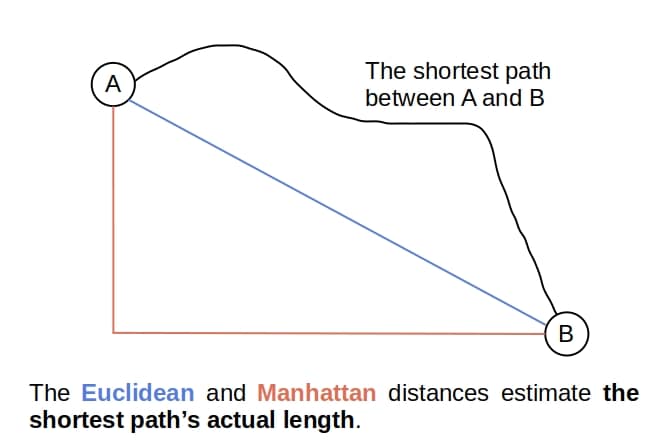
A heuristic  is a function that receives a state and outputs an estimate of the optimal path’s cost from to the closest goal. For example, if the states represent points on a 2D map, the Euclidean and Manhattan distances are good candidates for heuristics:
However, the use of heuristics is not the only difference between Dijkstra and A*.
4.2. The Frontier
A* differs from UCS only in the ordering of its frontier. UCS orders the nodes in the frontier by their values. They represent the costs of the paths from the start state to the frontier nodes’ states. In A*, we order the frontier by  . If is an arbitrary node in the frontier, we interpret the value of
  as the estimated cost of the optimal path that connects the start and the goal and passes through the ‘s state.
Now, confusion may arise because we defined  as taking a state as its input but now give it a search node. The difference is only technical, because we can define
  .
.
5. The Difference in Assumptions
Dijkstra has two assumptions:
- the graph is finite
- the edge costs are non-negative
The first assumption is necessary because Dijkstra places all the nodes into at the beginning. If the second assumption doesn’t hold, we should use the Bellman-Ford algorithm. The two assumptions ensure that Dijkstra always terminates and returns either the optimal path or a notification that no goal is reachable from the start state.
It’s different for A*. The following two assumptions are necessary for the algorithm to terminate always:
- the edges have strictly positive costs

- the state graph is finite, or a goal state is reachable from the start
So, A* can handle an infinite graph if all the graph’s edges are positive and there’s a path from the start to a goal. But, there may be no zero-cost edges even in the finite graphs. Further, there are additional requirements that A* should fulfill so that it returns only the optimal paths. We call such algorithms optimal.
5.1. Optimality of A*
First, we should note that A* comes in two flavors: the Tree-Like Search (TLS) and the Graph-Search (GS). TLS doesn’t check for repeated states, whereas GS does.
If we don’t check for repeated states and use the TLS A*, then should be admissible for the algorithm to be optimal. We say that a heuristic is admissible if it never overestimates the cost to reach the goal. So, if  is the actual cost of the optimal path from
  to the goal, then is admissible if
  for any . Even inadmissible heuristics may lead us to the optimal path or even give us an optimal algorithm, but there are no guarantees for that.
If we want to avoid repeated states, we use the GS A*, and to make it optimal, we have to use consistent heuristics. A heuristic is consistent if it fulfills the following condition for any node and its child  :
:
![\[h(u) \leq c(u, v) + h(v)\]](/wp-content/ql-cache/quicklatex.com-2cf82e1ab6acdb0ed777b2e9b3bd7623_l3.svg "Rendered by QuickLaTeX.com")
where  is the cost of the edge
  in the state graph. A consistent heuristic is always admissible, but the converse doesn’t necessarily hold.
6. Search Trees and Search Contours
Both Dijkstra’s Algorithm and A* superimpose a search tree over the graph. Since paths in trees are unique, each node in the search tree represents both a state and a path to the state. So, we can say that both algorithms maintain a tree of paths from the start state at each point in their execution. However, Dijkstra and A* differ by the order in which they include the nodes in their trees.
We can visualize the difference by drawing the search wavefronts over the graph. We define each wave as the set of nodes having the path cost in the range ![[C', C'']](/wp-content/ql-cache/quicklatex.com-3a4aba0c89bf6d2764d4face16eeda53_l3.svg "Rendered by QuickLaTeX.com") when added to the tree, where we choose the border values and
when added to the tree, where we choose the border values and  in advance. If we suitably select the incremental values
  to define the waves, they’ll show us how the search progresses through the graph.
6.1. Dijkstra
The search tree’s root is , and its nodes are the vertices in . Because of the invariant, we know that the nodes represent the optimal paths. The edge non-negativity assumption, together with the policy of choosing the lowest-cost node to move from to , ensures another property of Dijkstra. It can move to a state whose optimal path costs more than  only after moving all the states whose optimal paths cost
  , for any .
So, the contours which separate the waves in Dijkstra look more or less like uniform circles:
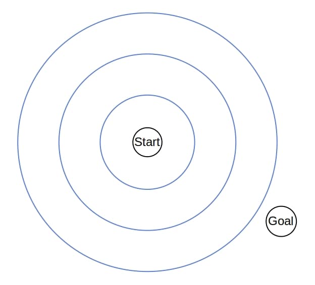
Therefore, the search tree of Dijkstra grows uniformly in all the directions in the topology induced by the graph.
6.2. A*
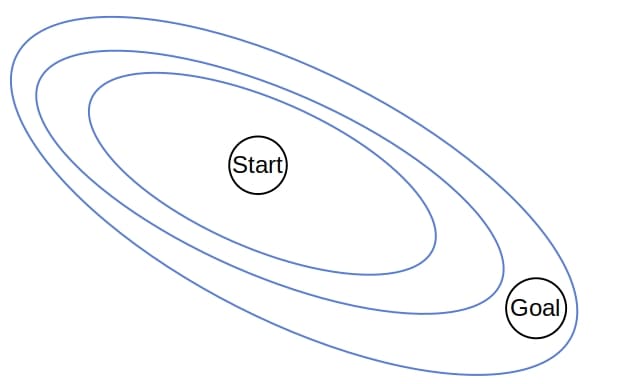
Whereas UCS and Dijskra spread through the state graph in all directions and have uniform contours, A* favors some directions over the others. Between two nodes with the same values, A* prefers the one with a better value. So, the heuristic stretches the contours in the direction of the goal state(s):
7. Differences in Complexity
Here, we’ll compare the space and time complexities of Dijkstra’s Algorithm and A*
7.1. Dijkstra
The worst-case time complexity depends on the graph’s sparsity and the data structure to implement . For example, in dense graphs,  , and since Dijkstra checks each edge twice, its worst-case time complexity is also
  .
.
However, if the graph is sparse,  is not comparable to
  . With a Fibonacci heap as , the time complexity becomes
  .
.
Since  , the space complexity is
  .
.
7.2. A*
The time and space complexities of GS A* are bounded from above by the state graphs’ size. In the worst-case, A* will require memory and have  time complexity, similar to Dijkstra and UCS. However, that’s the worst-case scenario. In practice, the search trees of A* are smaller than those of Dijkstra and UCS. That’s because the heuristics usually prune large portions of the tree that Dijkstra would grow on the same problem. For those reasons, A* focuses on the promising nodes in the frontier and finds the optimal path faster than Dijkstra or UCS.
The worst-case time of TLS A* is  , where
  is the upper bound of the branching factor, is the optimal path’s cost, and
  is the minimal edge cost. However, its effective complexity isn’t as bad in practice because A* reaches fewer nodes. The same goes for the space complexity of TLS A*.
8. The Hierarchy of Algorithms
In a way, Dijkstra is an instance of A*. If we use a trivial heuristic that always returns 0, A* reduces to UCS. But, UCS is equivalent to Dijkstra in the sense that they have the same search trees. So, we can simulate Dijkstra with an A* that uses  as the heuristic.
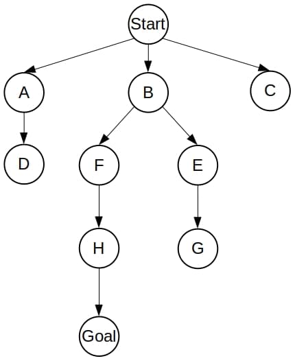
9. Example
Let’s see how Dijkstra and A* would find the optimal path between  and
and  in the following graph:
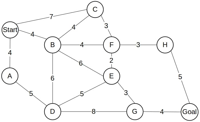
The search tree of Dijkstra spans the whole graph:
However, if we use the following heuristic estimates:
![\[\begin{aligned} h(A) = 13 && h(B) = 10 && h(C) = 10 && h(D) = 9 \\ h(E) = 7 && h(F) = 7 && h(G) = 2 && h(H) = 3 \\ h(Start) = 15 && h(Goal) = 0 && \end{aligned}\]](/wp-content/ql-cache/quicklatex.com-69c0c1091eb2384faee008f7221ffc50_l3.svg "Rendered by QuickLaTeX.com")
the tree of A* will contain only the optimal path:
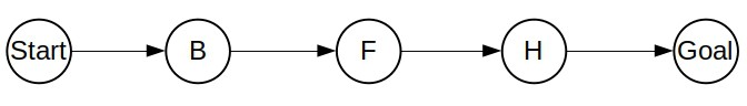
which means that A* won’t expand any unnecessary node!
10. Summary
So, here’s the summary of Dijkstra vs. A*.
| Dijkstra | A* | |
|---|---|---|
| Graph | finite | both finite and infinite graphs |
| Edge costs | non-negative | strictly positive |
| Time complexity | or |
 or or |
| Space complexity | |
or |
| Search contours | uniform | stretched toward the goal(s) |
| In practice | slower than A* | fast if the heuristic is good |
| Computing | inside the algorithm | heuristics incur computational overhead |
| Input | require only the problem definition | designing a good heuristic requires time |
As we see, the efficiency of A* stems from the properties of the heuristic function used. So, implementations of A* require an additional step of designing a quality heuristic. It has to guide the search efficiently through the graph but also be computationally lightweight.
11. Conclusion
In this article, we talked about Dijkstra’s Algorithm and A*. We presented their differences and explained why the latter is faster in practice.