Comparison Between Uniform-Cost Search and Dijkstra’s Algorithm

1. Introduction

In graph theory, the shortest path problem is about finding a path between two vertices in a graph such that the total sum of the path edge weights is minimum. We can use both Dijkstra’s algorithm and the uniform-cost search algorithm to find the shortest paths between vertices in a graph.

In this tutorial, we’ll introduce these two algorithms and compare them.

2. General Dijkstra’s Algorithm

Given a source vertex $\mathbf {s}$ in a weighted directed graph $\mathbf{G = (V, E)}$ where all edge weights are non-negative, Dijkstra’s algorithm can find the shortest path between $\mathbf{s}$ and every other vertex in $\mathbf{G}$ . Let’s first start with a general framework of the Dijkstra’s algorithm:

algorithm Dijkstra(G, s):
    // INPUT
    //     G = weighted directed graph (G = (V, E))
    //     s = the source vertex
    // OUTPUT
    //     dist = the shortest paths' weights from s to all vertices

    for v in V:
        dist[v] <- +infinity
    dist[s] <- 0
    Q <- empty vertex set
    for v in V:
        add v to Q with key dist[v]

    while Q is not empty:
        u <- the vertex in Q with smallest dist[u]
        
        remove u from Q
        visited[u] <- true
        if dist[u] == +infinity:
            break

        for v in Adj(u) and not visited[v]:
            dist <- dist[u] + w(u, v)
            if dist < dist[v]:
                dist[v] <- dist
                update Q for vertex v

    return dist

In this algorithm, we first set zero distance to our initial vertex and infinity to all other vertices. Also, we start with an initial vertex set, $Q$ , which contains all vertices in the graph $G$ .

At every iteration of the loop, we first extract the vertex $u \in Q$ with the minimal distance value. Then, for each unvisited neighbor $v$ of $u$ , we update its distance value with formula $dist[v] = min(dist[v], dist[u] + w(u, v))$ , where $w(u,v)$ is the weight of edge $(u,v)$ . In the end, for each vertex $v \in V$ , $dist[v]$ contains the shortest path weight between $s$ and $v$ .

The time complexity of Dijkstra’s algorithm depends on how we implement $Q$ .

If we use a min-priority queue with binary min-heap, each extraction takes $O(log|V|)$ time, where $|V|$ is the number of vertices in $G$ . There are $|V|$ such operations. Also, we need to update the priority queue when we change the distance value of an adjacent vertex. Each update operation takes $O(log|V|)$ time. There are at most $|E|$ such operations, where $|E|$ is the number of edges in $G$ .

Therefore, the overall time complexity of Dijkstra’s algorithm is $\mathbf {O((|V| + |E|)log|V|)}$ .

3. Dijkstra’s Algorithm for Single-Pair Shortest Path Problem

The general Dijkstra’s algorithm can find the shortest path between the source vertex $s$ and every other vertex in $G$ . In some applications, we only want to find the shortest path between a source vertex $s$ and a destination vertex $d$ .

It is easy to extend the general Dijkstra’s algorithm to solve this single-pair shortest path problem. Firstly, we can stop the loop when we see the extracted vertex $u$ is our destination vertex $d$ . Secondly, we can use a new data structure $prev$ to record the previous vertex along the shortest path. In this way, we can build the whole shortest path after we finish the loop:

algorithm DijkstraPair(G, s, d):
    // INPUT
    //     G = (V, E) = a weighted directed graph
    //     s = the source vertex
    //     d = the destination vertex
    // OUTPUT
    //     The list of vertices on the shortest path between s and d

    for v in V:
        dist[v] <- +infinity
    dist[s] <- 0
    Q <- empty vertex set
    for v in V:
        add v to Q with key dist[v]

    while Q is not empty:
        u <- find the vertex in Q with smallest dist[u]
        remove u from Q
        if u = d:
            break
        visited[u] <- true
        if dist[u] = +infinity:
            break

        for v in Adj(u) and not visited[v]:
            dist <- dist[u] + w(u, v)
            if dist < dist[v]:
                dist[v] <- dist
                update Q for vertex v
                prev[v] <- u

    return buildPath(s, d, prev)

In the $buildPath$ function, we start with the destination vertex $d$ and gradually add the previous vertices into the path based on the data in the $prev$ . We stop building the path once we reach the source vertex $s$ :

algorithm buildPath(s, d, prev):
    // INPUT
    //     s = the source vertex
    //     d = the destination vertex
    //     prev = the map of previous vertices in shortest path
    // OUTPUT
    //     The path from s to d

    path <- create an empty list
    v <- d
    while v != s:
        insert v at the front of path
        v <- prev[v]
    insert s at the front of path

    return path

4. Uniform-Cost Search Algorithm

Best-first search is a search algorithm that traverses a graph by expanding the most promising vertex based on a specified rule. The uniform-cost search algorithm is a simple version of the best-first search scheme, where we only evaluate the cost to the start vertex when we choose a vertex to expand.

We can also use the uniform-cost search algorithm to find the shortest path between a source vertex $s$ and every other vertex in graph $G$ . In this algorithm, we first start with a single vertex $s$ and then gradually expand to other vertices. Similar to Dijkstra’s algorithm, we choose a vertex whose distance to $s$ is minimum in each expanding step.

4.1. Flowchart and Pseudocode

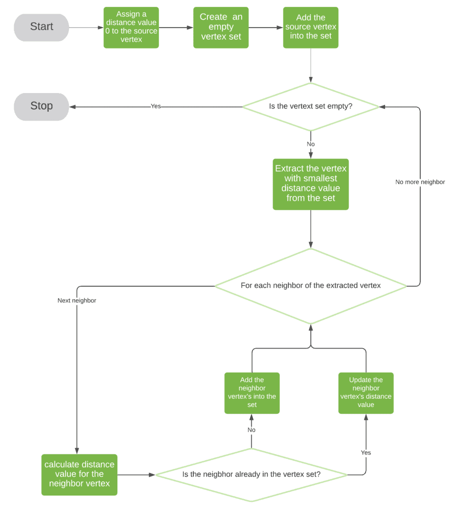
In this algorithm, we start with an initial vertex set, $Q$ , which only contains the start vertex $s$ . Then, we use a loop to process vertices inside $Q$ to calculate the shortest paths from the start vertex to all the other vertices in $G$ .

At every iteration of the loop, we first extract the vertex $u \in Q$ with the minimal distance value. Then, for each neighbor $v$ of $u$ , we calculate its distance value with formula $dist[v] = min(dist[v], dist[u] + w(u, v))$ , where $w(u,v)$ is the weight of edge $(u,v)$ . If the neighbor vertex is already in the $Q$ , we just update its associated distance value. Otherwise, we add the neighbor vertex into $Q$ .

We keep this looping process until $Q$ is empty. The time complexity of the uniform-cost algorithm is also $O((|V| + |E|)log|V|)$ , if we use a min-priority queue to implement $Q$ .

We can translate the flowchart of the uniform-cost search algorithm into the pseudocode:

algorithm UniformCost(G, s):
    // INPUT
    //     G = (V, E) = a weighted directed graph
    //     s = the source vertex
    // OUTPUT
    //     dist = the shortest paths' weights from s to all vertices

    dist[s] <- 0
    Q <- create an empty vertex set
    add s to Q with key dist[s]

    while Q is not empty:
        u <- find the vertex in Q with smallest dist[u]
        
        remove u from Q

        for v in Adj(u):
            dist <- dist[u] + w(u, v)
            if v in Q:
                if dist < dist[v]:
                    dist[v] <- dist
                    update Q for vertex v
            else:
                dist[v] <- dist
                add v to Q with key dist[v]

    return dist

4.2. Uniform-Cost Algorithm for Single-Pair Shortest Path Problem

Similarly, we can extend the uniform-cost algorithm to solve the single-pair shortest path problem:

algorithm UniformCostPair(G, s, d):
    // INPUT
    //     G = (V, E) = a weighted directed graph
    //     s = the source vertex
    //     d = the destination vertex
    // OUTPUT
    //     The path from s to d

    dist[s] <- 0
    Q <- create an empty vertex set
    add s to Q with key dist[s]

    while Q is not empty:
        u <- find the vertex in Q with smallest dist[u]
        
        remove u from Q
        if u = d:
            break

        for v in Adj(u):
            dist <- dist[u] + w(u, v)
            if v in Q:
                if dist < dist[v]:
                    dist[v] <- dist
                    prev[v] <- u
                    update Q for vertex v
            else:
                dist[v] <- dist
                add v to Q with key dist[v]
                prev[v] <- u

    return buildPath(s, d, prev)

In this algorithm, we stop the loop when we see the extracted vertex $u$ is our destination vertex $d$ . Also, we use a data structure $prev$ to record the previous vertex along the shortest path. In the end, we call the $buildPath$ function to construct the shortest path.

5. Comparison Between Uniform-Cost Search and Dijkstra’s Algorithm

Both Dijkstra’s algorithm and the uniform-cost algorithm can solve the shortest path problem with the same time complexity. They have similar code structures. Also, we use the same formula, $dist[v] = min(dist[v], dist[u] + w(u, v))$ , to update the distance value of each vertex.

The main difference between these two algorithms is how we store vertices in $Q$ . In Dijkstra’s algorithm, we initialize $Q$ with all vertices in $G$ . Therefore, Dijkstra’s algorithm is only applicable for explicit graphs where we know all vertices and edges.

However, the uniform-cost search algorithm starts with the source vertex and gradually traverses the necessary graph parts. Therefore, it is applicable for both explicit graphs and implicit graphs.

For the single-pair shortest path problem, Dijkstra’s algorithm has more memory requirements as we store the entire graph in memory. By contrast, the uniform-cost search algorithm only stores the source vertex at the beginning and stops expanding once we reach the destination vertex. Therefore, the uniform-cost search algorithm may only store a partial graph in the end.

Although both algorithms have the same time complexity on the single-pair shortest path problem, Dijkstra’s algorithm can be more time consuming due to memory requirements.

When we implement $Q$ with a min-heap priority queue, each queue operation takes $O(log n)$ time, where $n$ is the number of vertices in $Q$ . Dijkstra’s algorithm puts all vertices into $Q$ at the beginning. For a large graph, its vertices will create a big overhead when performing operations on $Q$ .

However, the uniform-cost search algorithm starts with a single vertex and gradually includes other vertices during the path building. Therefore, we’ll work on a much smaller number of vertices when we do priority queue operations.

Another small difference between these two algorithms is the final distance values on vertices that are not reachable from the source vertex. In Dijkstra’s algorithm, if there is no path between the source vertex $s$ and a vertex $v$ , its distance value ( $dist[v]$ ) is $+\infty$ . However, in the uniform-cost search algorithm, we cannot find such value in the final distance map, i.e., $dist[v]$ does not exist.

We can use a table to summarize our comparison results:

$\begin{tabular} {|c |c |c |c |c|} \hline &\bf{Initialization} & \bf{Memory Requirement} & \bf{Running Time} & \bf{Application}\\ \hline \bf{Dijkstra's algorithm} & A set of all vertices in \it{G} & Need to store the whole graph & Slower due to large memory requirement & Explicit graphs only \\ \hline \bf{Uniform-cost search algorithm} & A set with only the source vertex & Only store necessary vertices & Faster due to less memory requirement & Implicit and explicit graphs \\ \hline \end{tabular}$

6. Conclusion

In this tutorial, we showed both Dijkstra’s algorithm and the uniform-cost search algorithm. Also, we extended both algorithms to solve the single-pair shortest path problem. By comparing these two algorithms, we can see that the uniform-cost search algorithm can perform better than Dijkstra’s algorithm on large graphs.

Full Archive

About Baeldung

Core Concepts

Operating Systems

Artificial Intelligence

Graph Theory

Latex