Bidirectional Search for Path Finding | Baeldung on Computer Science

1. Introduction

In this tutorial, we’ll talk about Bidirectional Search (BiS). It’s an algorithm for finding the shortest (or the lowest-cost) path between the start and end nodes in a graph.

2. Search

Classical AI search algorithms grow a search tree over the graph at hand. The tree root is the start node, and it grows as the search algorithm visits other vertices. The algorithms stop after reaching the target node and including it in the tree. Breadth-First Search (BFS), Depth-First Search, Uniform-Cost Search (UCS), and A* are examples of such algorithms. They’re all instances of Best-First Search, which is unidirectional: the search spreads in waves from the single node and forms a tree.

2.1. Motivation for Bidirectional Search (BiS)

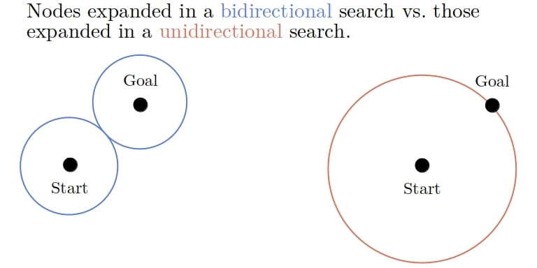
That’s a straightforward but not necessarily the best way to search for the best path. Let’s take a look at BFS. Its tree-like version has the $O(b^d)$ worst-case time and space complexities, where $b$ is the upper bound of the branching factor, and $d$ is the depth of the shallowest goal node. However, if we start the search from the goal node as well, we’ll have two trees with potentially fewer nodes.

The two trees in Bidirectional BFS grow simultaneously in opposite directions. The forward search tree grows from the start node and tries to reach the goal node, as before. But, the reverse search tree grows from the goal as its root and tries to reach the start. When the two trees meet, we’ve got the shortest path between the start and goal vertices (under certain conditions). But, the total number of nodes in the trees is expected to be lower than if we grew a single tree from the start node:

To see why that is, let’s imagine that the trees meet at the middle node on the path from the start to the goal. Then, the trees together contain at most $O(b^{d/2})$ nodes. With a constant branching factor $b=10$ and $d=20$ , unidirectional BFS would grow a tree with $10^{20}$ nodes in the worst-case scenario, whereas BiBFS’s trees would contain $2\cdot 10^{20/2}=2\cdot 10^{10}$ nodes together. That’s five billion times fewer nodes.

2.2. Base Algorithms for Bidirectional Search

BiS is a generic search technique. We can use any unidirectional algorithm to run the forward search and combine it with any single-source algorithm for the reverse search. They can but need not be the same. That means that BiS describes a plethora of methods we obtain by combining different base algorithms for the forward and reverse searches.

3. Reverse Edges

A directed edge from $u$ to $v$ represents an action the AI agent should take to get from $u$ to $v$ . However, the reverse search goes in the opposite direction, so it requires the reversal of all the edges in the graph. Therefore, to run a BiS, we have to traverse the graph in both directions.

Unlike the original forward edges, their reverse counterparts can but don’t have to denote actions. A reverse edge from $v$ to $u$ means that there is an action that leads from $u$ to $v$ . There need not be a real-world action that leads from $v$ to $u$ for the reverse arc $v \rightarrow u$ to exist. Reversal needs only to be computationally possible.

For example, if time is a feature of the nodes, and each forward action has a non-zero duration, then reverse actions will be impossible (unless we’ve got a time machine). Nevertheless, if we’re able to define them computationally, we can use BiS.

4. Bidirectional UCS

When making a case for Bidirectional Search, we said we aimed for the forward and reverse searches to meet somewhere in the graph. That means that they both have reached the same node. However, there are other things we should know to implement a bidirectional algorithm:

Should we alternate between the searches? If yes, how?
Does the optimal path necessarily pass through the meeting point?

We’ll answer both questions on the example of Bidirectional UCS (BiUCS).

4.1. Alternation

Conceptually, we are running two searches in parallel. But, in practice, we can’t execute both at the same time on the same CPU. What we can do is interleave the forward and reverse searches.

Let’s define a search step as the body of the main unidirectional UCS loop. In BiUCS, we also have a single main loop, but in each iteration, we choose which search to advance. One strategy could be to alternate between the searches: run a forward, then reverse, then forward again, then reverse again, and so on. The other way would be to execute a step of the search whose frontier’s top node is closer to its source (the start or the goal). Which one is better?

The latter strategy is more consistent with the spirit of unidirectional UCS, and that is to expand the frontier node that’s closest to the source. Since we have two frontiers in BiUCS, we choose the node closer to its frontier’s source. But, the strategy may degenerate to running the search in one direction only. For example, if the edges’ costs exponentially increase with the proximity to the goal, we may not execute any reverse step. To avoid this scenario, we can alternate between the searches by following each forward step by reverse and each reverse step by a forward one. Still, both strategies will work under the stopping criterion we describe next.

4.2. Stopping Condition

We said that the aim of bidirectional search was for the forward and reverse searches to meet at some node $u$ . Algorithmically, that’s the point when we reach $u$ in one direction after expanding it in the other search. But should we stop the whole algorithm at that point and claim we’ve found the optimal path (through $u$ )?

Just as we shouldn’t stop unidirectional UCS after adding a goal node to the frontier, we shouldn’t terminate the bidirectional variant if a node $u$ is expanded in one search and put into the frontier in the other. The reason is that there may be a lower-cost path to $u$ from the source of the second frontier it’s been added to.

So, what’s the correct stopping condition? Let’s say that $\mu$ is the cost of the best path we’ve found so far (initially, we set it to $\infty$ ). Whenever we reach a node we’ve expanded in the other search, we update $\mu$ if a better path goes through the node. Let $g_F$ be the current distance from the start and $g_R$ the current distance from the goal node. Let $top_F$ and $top_R$ be the distances to the top nodes in the forward and reverse frontier queues, respectively. Then, we can stop the algorithm if:

$top_F + top_R \geq \mu$

4.3. Correctness of the Stopping Condition

Let’s suppose that the stopping condition $top_F + top_R \geq \mu$ has obtained. For any node $u$ unexpanded in the forward search, it holds that $g_F^*(u) \geq top_F$ , where $g_F^*$ is the actual distance from the start. Similar holds if $u$ is unexpanded in the reverse search: $g_R^*(u) \geq top_R$ , where $g_R^*$ is the actual distance from the goal.

Now, let’s suppose that we’ve expanded a node $u$ at a subsequent forward step and that its successor $v$ has already been expanded in the reverse search. The path through $u$ and $v$ will cost $g_F^*(v) + g_R^*(v)$ where:

$g_F^*(v) \geq top_F$

because we’ve added $v$ to the forward frontier and will expand it later, and:

$g_R^*(v) \geq top_R$

because we’ve expanded $v$ after the stopping condition. So the path’s cost will be $\geq top_F + top_R \geq \mu$ .

In the other case, we expanded $v$ in the reverse search before the stopping condition was obtained, so we can’t conclude that $g_R^*(v) \geq top_R$ . However, since $u$ has not been reverse-expanded yet, we know that $g_R^*(u) \geq top_R$ . The path’s cost is also $g_F^*(u) + g_R^*(u)$ , so we have:

$g_F^*(u) + g_R^*(u) \geq top_F + top_R \geq \mu$

Therefore, $\mu$ is the cost of the optimal path, which proves the correctness of the stopping condition.

4.4. Pseudocode of Bidirectional Search

Finally, here’s the pseudocode of BiUCS:

The $STEP$ function is responsible for advancing the searches through the graph and updating $\mu$ . Here’s how it works:

5. Discussion

BiS is possible only if we have explicit goal nodes. If we only have a goal test, then we can’t run the reverse search. That’s also the case if the reverse edges aren’t computationally tractable.

Having more than one goal node isn’t a problem as long as they’re all explicit. Which one do we choose as the source of the reverse search? Neither. We construct an artificial goal node, link it to the actual goals with zero-cost edges, and set it as the reverse source.

BiS is expected to find the optimal path faster than a unidirectional search but is harder to implement and debug. While possible, combining different algorithms for forward and reverse searches may not be justified. If all the edges have constant costs, our best choices are BFS or Iterative Deepening for both searches. In the case that the edge costs differ, we should bidirectionalize UCS or A*.

Finally, the stopping condition may be difficult to formulate and prove. If we design it right, our BiS can be both optimal and complete. The former means that it cannot return a suboptimal path, whereas the latter means that it always terminates returning either a path or a notification of failure. The stopping condition depends on the base algorithms.

6. Conclusion

In this article, we presented generic Bidirectional Search (BiS) and Bidirectional UCS (BiUCS). BiS is a generic search algorithm that runs two unidirectional algorithms in parallel: one that grows its search tree from the start to the goal, and the other that does so from the goal to the start. In general, we expect BiS to find the optimal path faster than single-source algorithms. But, it requires careful design, especially concerning the stopping criteria, and is harder to implement and debug.

Full Archive

About Baeldung

Core Concepts

Operating Systems

Artificial Intelligence

Graph Theory

Latex