Spark DataFrame

1. Overview

Apache Spark is an open-source and distributed analytics and processing system that enables data engineering and data science at scale. It simplifies the development of analytics-oriented applications by offering a unified API for data transfer, massive transformations, and distribution.

The DataFrame is an important and essential component of Spark API. In this tutorial, we’ll look into some of the Spark DataFrame APIs using a simple customer data example.

2. DataFrame in Spark

Logically, a DataFrame is an immutable set of records organized into named columns. It shares similarities with a table in RDBMS or a ResultSet in Java.

As an API, the DataFrame provides unified access to multiple Spark libraries including Spark SQL, Spark Streaming, MLib, and GraphX.

In Java, we use Dataset<Row> to represent a DataFrame.

Essentially, a Row uses efficient storage called Tungsten, which highly optimizes Spark operations in comparison with its predecessors.

3. Maven Dependencies

Let’s start by adding the spark-core and spark-sql dependencies to our pom.xml:

<dependency>
    <groupId>org.apache.spark</groupId>
    <artifactId>spark-core_2.11</artifactId>
    <version>2.4.8</version>
</dependency>

<dependency>
    <groupId>org.apache.spark</groupId>
    <artifactId>spark-sql_2.11</artifactId>
    <version>2.4.8</version>
</dependency>

4. DataFrame and Schema

Essentially, a DataFrame is an RDD with a schema. The schema can either be inferred or defined as a StructType.

StructType is a built-in data type in Spark SQL that we use to represent a collection of StructField objects.

Let’s define a sample Customer schema StructType:

public static StructType minimumCustomerDataSchema() {
    return DataTypes.createStructType(new StructField[] {
      DataTypes.createStructField("id", DataTypes.StringType, true),
      DataTypes.createStructField("name", DataTypes.StringType, true),
      DataTypes.createStructField("gender", DataTypes.StringType, true),
      DataTypes.createStructField("transaction_amount", DataTypes.IntegerType, true) }
    );
}

Here, each StructField has a name that represents the DataFrame column name, type, and boolean value that represents whether it’s nullable.

5. Constructing DataFrames

The first operation for every Spark application is to get a SparkSession via master.

It provides us with an entry point to access the DataFrames. Let’s start by creating the SparkSession:

public static SparkSession getSparkSession() {
    return SparkSession.builder()
      .appName("Customer Aggregation pipeline")
      .master("local")
      .getOrCreate();
}

Note here that we’re connecting to Spark using the local master. If we were to connect to the cluster, we would give the cluster address instead.

Once we have a SparkSession, we can create a DataFrame using various methods. Let’s briefly look at some of them.

5.1. DataFrame from List<POJO>

Let’s build a List<Customer> first: 

List<Customer> customers = Arrays.asList(
  aCustomerWith("01", "jo", "Female", 2000), 
  aCustomerWith("02", "jack", "Male", 1200)
);

Next, let’s construct the DataFrame from the List<Customer> using createDataFrame:

Dataset<Row> df = SPARK_SESSION
  .createDataFrame(customerList, Customer.class);

5.2. DataFrame from Dataset

If we have a Dataset, we can easily convert it to a DataFrame by calling toDF on the Dataset.

Let’s create a Dataset<Customer> first, using createDataset, that takes org.apache.spark.sql.Encoders:

Dataset<Customer> customerPOJODataSet = SPARK_SESSION
  .createDataset(CUSTOMERS, Encoders.bean(Customer.class));

Next, let’s convert it to DataFrame:

Dataset<Row> df = customerPOJODataSet.toDF();

5.3. Row from a POJO Using RowFactory

Since DataFrame is essentially a Dataset<Row>, let’s see how we can create a Row from a Customer POJO.

Basically, by implementing MapFunction<Customer, Row> and overriding the call method, we can map each Customer to a Row using RowFactory.create:

public class CustomerToRowMapper implements MapFunction<Customer, Row> {
    
    @Override
    public Row call(Customer customer) throws Exception {
        Row row = RowFactory.create(
          customer.getId(),
          customer.getName().toUpperCase(),
          StringUtils.substring(customer.getGender(),0, 1),
          customer.getTransaction_amount()
        );
        return row;
    }
}

We should note that we can manipulate the Customer data here before converting it into a Row.

5.4. DataFrame from List<Row>

We can also create a DataFrame from a list of Row objects:

List<Row> rows = customer.stream()
  .map(c -> new CustomerToRowMapper().call(c))
  .collect(Collectors.toList());

Now, let’s give this List<Row> to SparkSession along with the StructType schema:

Dataset<Row> df = SparkDriver.getSparkSession()
  .createDataFrame(rows, SchemaFactory.minimumCustomerDataSchema());

Note here that the List<Row> will be converted to DataFrame based on the schema definition. Any field not present in the schema will not be part of the DataFrame.

5.5. DataFrame from Structured Files and Database

DataFrames can store columnar information, like a CSV file, and nested fields and arrays, like a JSON file.

The DataFrame API remains the same regardless of whether we’re working with CSV files, JSON files, or other formats as well as Databases.

Let’s create the DataFrame from multiline JSON data:

Dataset<Row> df = SparkDriver.getSparkSession()
  .read()
  .format("org.apache.spark.sql.execution.datasources.json.JsonFileFormat")
  .option("multiline", true)
  .load("data/minCustomerData.json");

Similarly, in the case of reading from the database, we’ll have:

Dataset<Row> df = SparkDriver.getSparkSession()
  .read()
  .option("url", "jdbc:postgresql://localhost:5432/customerdb")
  .option("dbtable", "customer")
  .option("user", "user")
  .option("password", "password")
  .option("serverTimezone", "EST")
  .format("jdbc")
  .load();

6. Converting DataFrame to Dataset

Now, let’s see how we can convert our DataFrame into a Dataset. This conversion is useful if we want to manipulate our existing POJOs and the extended API that apply to only the DataFrame.

We’ll continue with the DataFrame created from JSON in the previous section.

Let’s call a mapper function that takes each row of the Dataset<Row> and converts it into a Customer object:

Dataset<Customer> ds = df.map(
  new CustomerMapper(),
  Encoders.bean(Customer.class)
);

Here, the CustomerMapper implements MapFunction<Row, Customer>:

public class CustomerMapper implements MapFunction<Row, Customer> {

    @Override
    public Customer call(Row row) {
        Customer customer = new Customer();
        customer.setId(row.getAs("id"));
        customer.setName(row.getAs("name"));
        customer.setGender(row.getAs("gender"));
        customer.setTransaction_amount(Math.toIntExact(row.getAs("transaction_amount")));
        return customer;
    }
}

We should note that the MapFunction<Row, Customer> is instantiated only once, whatever the number of records we have to process.

7. DataFrame Operations and Transformations

Now, let’s build a simple pipeline using a customer data example. We want to ingest customer data as DataFrames from two disparate file sources, normalize them, and then perform some transformations on the data.

Finally, we’ll write the transformed data to a database.

The purpose of these transformations is to find out the yearly spending, ordered by gender and source.

7.1. Ingesting Data

Firstly, let’s ingest data from a couple of sources using SparkSession‘s read method starting with JSON data:

Dataset<Row> jsonDataToDF = SPARK_SESSION.read()
  .format("org.apache.spark.sql.execution.datasources.json.JsonFileFormat")
  .option("multiline", true)
  .load("data/customerData.json");

Now, let’s do the same with our CSV source:

Dataset<Row> csvDataToDF = SPARK_SESSION.read()
  .format("csv")
  .option("header", "true")
  .schema(SchemaFactory.customerSchema())
  .option("dateFormat", "m/d/YYYY")
  .load("data/customerData.csv"); 

csvDataToDF.show(); 
csvDataToDF.printSchema(); 
return csvData;

Importantly, to read this CSV data, we’re providing a StructType schema that determines the column data types.

Once we’ve ingested the data, we can inspect the contents of the DataFrame using the show method.

Additionally, we can also limit the rows by providing the size in the show method. And, we can use printSchema to inspect the schemas of the newly created DataFrames.

We’ll notice that the two schemas have some differences. Therefore, we need to normalize the schema before we can do any transformations.

7.2. Normalizing DataFrames

Next, we’ll normalize the raw DataFrames representing the CSV and JSON data.

Here, let’s see some of the transformations performed:

private Dataset<Row> normalizeCustomerDataFromEbay(Dataset<Row> rawDataset) {
    Dataset<Row> transformedDF = rawDataset
      .withColumn("id", concat(rawDataset.col("zoneId"),lit("-"), rawDataset.col("customerId")))
      .drop(column("customerId"))
      .withColumn("source", lit("ebay"))
      .withColumn("city", rawDataset.col("contact.customer_city"))
      .drop(column("contact"))
      .drop(column("zoneId"))
      .withColumn("year", functions.year(col("transaction_date")))
      .drop("transaction_date")
      .withColumn("firstName", functions.split(column("name"), " ")
        .getItem(0))
      .withColumn("lastName", functions.split(column("name"), " ")
        .getItem(1))
      .drop(column("name"));

    return transformedDF; 
}

Some important operations on DataFrame in the above example are:

• concat to join data from multiple columns and literals to make a new id column
• lit static function returns a column with a literal value
• functions. year to extract the year from transactionDate
• function.split to split name into firstname and lastname columns
• drop method removes a column in the data frame
• col method returns a dataset’s column based on its name
• withColumnRenamed returns a column with renamed value

Importantly, we can see that the DataFrame is immutable. Hence, whenever anything needs to change, we must create a new DataFrame.

Eventually, both data frames are normalized to the same schema as below:

root
 |-- gender: string (nullable = true)
 |-- transaction_amount: long (nullable = true)
 |-- id: string (nullable = true)
 |-- source: string (nullable = false)
 |-- city: string (nullable = true)
 |-- year: integer (nullable = true)
 |-- firstName: string (nullable = true)
 |-- lastName: string (nullable = true)

7.3. Combining DataFrames

Let’s combine the normalized DataFrames next:

Dataset<Row> combineDataframes(Dataset<Row> df1, Dataset<Row> df2) {
    return df1.unionByName(df2); 
}

Importantly, we should note that:

• If we care about column names when we union two DataFrames, we should use unionByName
• If we don’t care about column names when we union two DataFrames, we should use union

7.4. Aggregating DataFrames

Next, let’s group the combined DataFrames to find out the yearly spending by year, source, and gender.

We’ll then sort the aggregated data by columns year ascending and yearly spent in descending order:

Dataset<Row> aggDF = dataset
  .groupBy(column("year"), column("source"), column("gender"))
  .sum("transactionAmount")
  .withColumnRenamed("sum(transaction_amount)", "yearly spent")
  .orderBy(col("year").asc(), col("yearly spent").desc());

Some important operations on DataFrame in the above example are:

• groupBy is used to arrange identical data into groups on DataFrame and then perform aggregate functions similar to SQL “GROUP BY” clause
• sum applies aggregation function on the column transactionAmount after grouping
• orderBy sorts the DataFrame by one or more columns
• asc and desc functions from Column class can be used to specify the sorting order

Finally, let’s use the show method to see what the data frame looks like after transformation:

+----+------+------+---------------+
|year|source|gender|annual_spending|
+----+------+------+---------------+
|2018|amazon|  Male|          10600|
|2018|amazon|Female|           6200|
|2018|  ebay|  Male|           5500|
|2021|  ebay|Female|          16000|
|2021|  ebay|  Male|          13500|
|2021|amazon|  Male|           4000|
|2021|amazon|Female|           2000|
+----+------+------+---------------+

Consequently, the schema after the final transformation should be:

root
 |-- source: string (nullable = false)
 |-- gender: string (nullable = true)
 |-- year: integer (nullable = true)
 |-- yearly spent: long (nullable = true)

7.5. Writing from DataFrame to a Relational Database

Finally, let’s finish off by writing the transformed DataFrame as a table in a relational database:

Properties dbProps = new Properties();

dbProps.setProperty("connectionURL", "jdbc:postgresql://localhost:5432/customerdb");
dbProps.setProperty("driver", "org.postgresql.Driver");
dbProps.setProperty("user", "postgres");
dbProps.setProperty("password", "postgres");

Next, we can use the Spark session to write to the database:

String connectionURL = dbProperties.getProperty("connectionURL");

dataset.write()
  .mode(SaveMode.Overwrite)
  .jdbc(connectionURL, "customer", dbProperties);

8. Testing

Now, we can test the pipeline end-to-end using the two ingestion sources, with postgres and pgAdmin Docker images:

@Test
void givenCSVAndJSON_whenRun_thenStoresAggregatedDataFrameInDB() throws Exception {
    Properties dbProps = new Properties();
    dbProps.setProperty("connectionURL", "jdbc:postgresql://localhost:5432/customerdb");
    dbProps.setProperty("driver", "org.postgresql.Driver");
    dbProps.setProperty("user", "postgres");
    dbProps.setProperty("password", "postgres");

    pipeline = new CustomerDataAggregationPipeline(dbProps);
    pipeline.run();

    String allCustomersSql = "Select count(*) from customer";

    Statement statement = conn.createStatement();
    ResultSet resultSet = statement.executeQuery(allCustomersSql);
    resultSet.next();
    int count = resultSet.getInt(1);
    assertEquals(7, count);
}

After running this, we can verify that a table exists with the columns and rows corresponding to the DataFrame. Finally, we can also observe this output via the pgAdmin4 client:

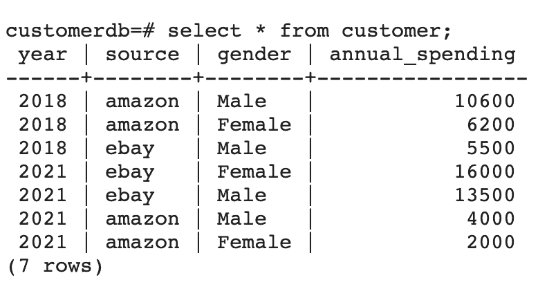
We should note a couple of important points here:

• The customer table is created automatically as a result of the write operation.
• The mode used is SaveMode.Overwrite. Consequently, this will overwrite anything already existing in the table. Other options available are Append, Ignore, and ErrorIfExists.

In addition, we can also use write to export DataFrame data as CSV, JSON, or parquet, among other formats.

9. Conclusion

In this tutorial, we looked at how to use DataFrames to perform data manipulation and aggregation in Apache Spark.

First, we created the DataFrames from various input sources. Then we used some of the API methods to normalize, combine, and then aggregate the data.

Finally, we exported the DataFrame as a table in a relational database.

As always, the full source code is available over on GitHub.