

Learn through the super-clean Baeldung Pro experience:
>> Membership and Baeldung Pro.
No ads, dark-mode and 6 months free of IntelliJ Idea Ultimate to start with.
Learn through the super-clean Baeldung Pro experience:
>> Membership and Baeldung Pro.
No ads, dark-mode and 6 months free of IntelliJ Idea Ultimate to start with.
In this tutorial, we’ll discuss two popular traffic controlling methods in TCP: flow and congestion control. First, we’ll present in detail how flow and congestion control works in TCP.
Finally, we’ll talk about the core differences between them.
Flow control deals with the amount of data sent to the receiver side without receiving any acknowledgment. It makes sure that the receiver will not be overwhelmed with data. It’s a kind of speed synchronization process between the sender and the receiver. The data link layer in the OSI model is responsible for facilitating flow control.
Let’s take a practical example to understand flow control. Jack is attending a training session. Let’s assume he’s slow in grasping concepts taught by the teacher. On the other hand, the teacher is teaching very fast without taking any acknowledgment from the students.
After some time, every word that comes out from his teacher is overflowing over Jack’s head. Hence, he doesn’t understand anything. Here, the teacher should be having information about how many concepts a student can handle at a time.
After some time, Jack requested the teacher to slow down the pace as he was overwhelmed with the data. The teacher decided to teach some of the concepts first and then wait for acknowledgment from the students before proceeding to the following concepts.
Similar to the example, the flow control mechanism tells the sender the maximum speed at which the data can be sent to the receiver device. The sender adjusts the speed as per the receiver’s capacity to reduce the frame loss from the receiver side.
Flow control in TCP ensures that it’ll not send more data to the receiver in the case when the receiver buffer is already completely filled. The receiver buffer indicates the capacity of the receiver. The receiver won’t be able to process the data when the receiver buffer is full:
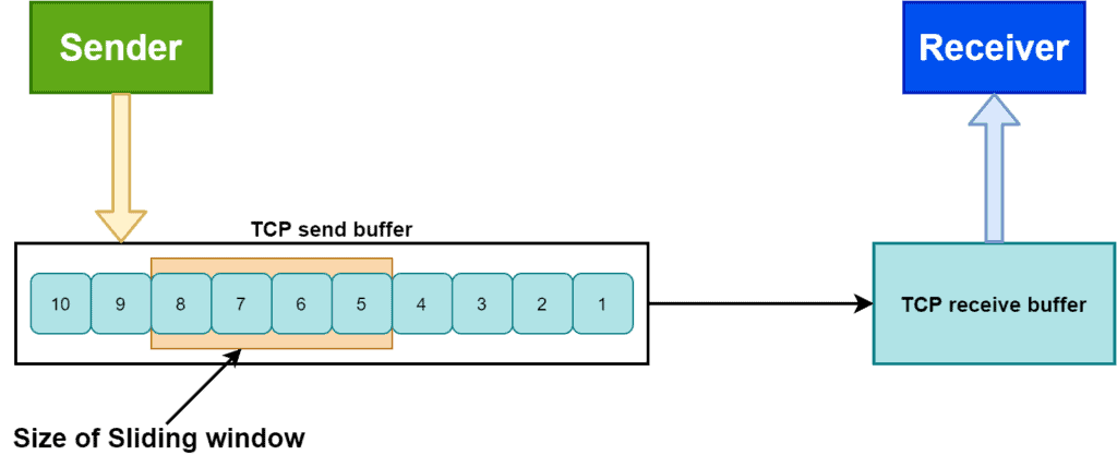
One of the popular flow control mechanisms in TCP is the sliding window protocol. It’s a byte-oriented process of variable size.
In this method, when we establish a connection between the sender and the receiver, the receiver sends the receiver window to the sender. The receiver window is the size that is currently available in the receiver’s buffer.
Now from the available receiver window, TCP calculates how much data can be sent further without acknowledgment. Although, if the receiver window size is zero, TCP halts the data transmission until it becomes a non-zero value.
The receiver window size is the part of the frame of TCP segments. The length of the window size is 16 bits, which means that the maximum size of the window is 65,535 bytes.
The receiver decides the size of the window. The receiver sends the currently available receiver window size with every acknowledgment message.
There are three processes in the sliding window protocol: opening window, closing window, shrinking window.
The opening window process allows more data to be in the buffer that can be sent:
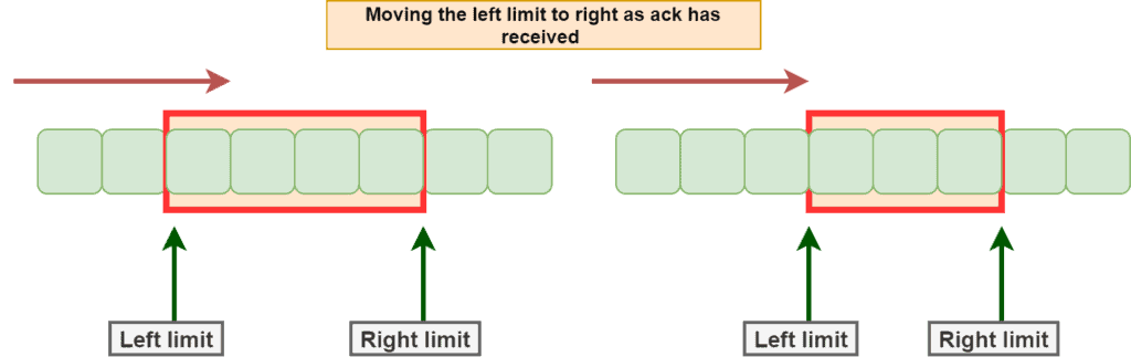
The closing window process indicates some sent data bytes have been acknowledged, and the sender needs not to worry about them anymore:

The shrinking windows process denotes the decrement in the window size. It means some bytes are eligible to transmit. Although because of the decrement in the window size, the sender won’t transfer those bytes. The receiver can open or close the window but shrinking the window is not recommended.
Suppose there are two devices: Device-A and Device-B. Device-A wants to send 300000 bytes of data to Device-B. Firstly, TCP breaks the data into small frames of size 1500 bytes each. Hence, there are 200 packets in total. In the beginning, let’s assume Device-B notifies the available receiver window to Device-A, which is 60000 bytes. It means Device-A can send 60000 bytes to Device-B without receiving the acknowledgment from Device-B.
Now Device-A can send up to 40 packets (1500*40 = 60000) without waiting for an acknowledgment. Therefore, Device-A has to wait for five acknowledgment messages to complete the whole transmission. The number of acknowledgment messages needed is calculated and by considering the receiver buffer’s capacity of Device-B:
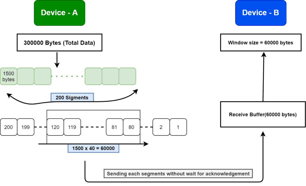
Here, TCP is responsible for arranging the data packets and making the window size 60000 bytes. Furthermore, TCP helps in transmitting the packets which fall in the window range from Device-A to Device-B. After sending the packets, it waits for the acknowledgment. If the acknowledgment has been received, it slides the window to the next 60000 bytes and sends the packets.
We know TCP stops the transmission when the receiver sends the zero-size window. However, there is a possibility that the receiver has sent an acknowledgment but was missed by the sender.
In that situation, the receiver waits for the next packet. But on the other hand, the sender is waiting for non-zero window size. Hence, this situation would result in a deadlock. To handle this case, TCP starts a persist timer when it receives a zero-window size. It also sends packets periodically to the receiver.
Congestion control is a mechanism that limits the flow of packets at each node of the network. Thus, it prevents any node from being overloaded with excessive packets. Congestion occurs when the rate of flow of packets towards any node is more than its handling capacity.
When congestion occurs, it slows down the network response time. As a result, the performance of the network decreases. Congestion occurs because routers and switches have a queue buffer, holding the packets for processing. After the holding process completes, they pass the packet to the next node, resulting in congestion in the network.
There are three phases that TCP uses for congestion control: slow start, congestion avoidance, and congestion detection:
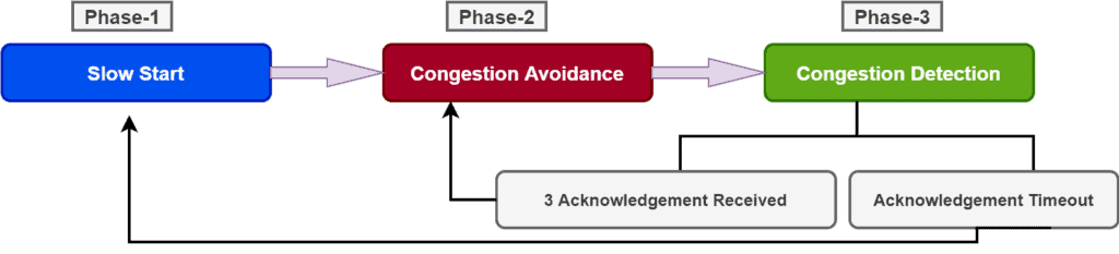
In the first phase of congestion control, the sender sends the packet and gradually increases the number of packets until it reaches a threshold. We know from the flow control discussion, the window size is decided by the receiver.
In the same way, there is a window size in the congestion control mechanism. It increases gradually. In the flow control, the window size (RWND) is sent with the TCP header. Although in congestion control, the sender node or the end device stores it.
The sender starts sending packets with window size (CWND) of 1 MSS (Max Segment Size). MSS denotes the maximum amount of data that the sender can send in a single segment. Initially, the sender sends only one segment and waits for the acknowledgment for segment 1. After that, the sender increases the window size (CWND) by 1 MSS each time.
The slow start process can’t continue for an indefinite time. Therefore, we generally use a threshold known as the slow start threshold (SSTHRESH) in order to terminate the slow start process. When the window size (CWND) reaches the slow-start threshold, the slow start process stops, and the next phase of congestion control starts. In most implementations, the value of the slow start threshold is 65,535 bytes.
The next phase of congestion control is congestion avoidance. In the slow start phase, window size (CWND) increases exponentially. Now, if we continue increasing window size exponentially, there’ll be a time when it’ll cause congestion in the network.
To avoid that, we use a congestion avoidance algorithm. The congestion avoidance algorithm defines how to calculate window size (CWND):
![\[Window Size (CWND) = Window Size (CWND) + Max Segment Size (MSS) / Window Size (CWND)\]](/wp-content/ql-cache/quicklatex.com-486ff061d8915599431ec68388387dd0_l3.svg "Rendered by QuickLaTeX.com")
After each acknowledgment, TCP ensures the linear increment in window size (CWND), slower than the slow start phase.
The third phase is congestion detection. Now in the congestion avoidance phase, we’ve decreased the rate of increment in window size (CWND) in order to reduce the probability of congestion in the network. If there is still congestion in the network, we apply a congestion detection mechanism.
There’re two conditions when TCP detects congestion. Firstly, when there is no acknowledgment received for a packet sent by the sender within an estimated time. The second condition occurs when the receiver gets three duplicate acknowledgments.
In the case of timeout, we start a new slow start phase. To handle the second situation, we begin a new congestion avoidance phase.
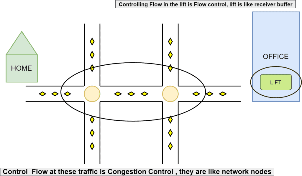
To summarize the flow and congestion control in TCP, let’s take a practical example.
Jack wakes up in the morning and gets ready for the office. On the way, he has to cross multiple road junctions, and there are traffic signals on each junction. In the office, there is a lift which drops him on his office floor.
In this example, all the traffic signals try to control the congestion from one junction to another. It works the same as maintaining the flow of segments from one node to another node in a network. Finally, when Jack reaches the office building, the flow control starts. The security guard controls access of the people for the lift as per the capacity of the lift. It’s like the receiver buffer concept inflow control:
Let’s talk about the core differences between flow and congestion control in TCP:
| Flow Control | Congestion Control |
|---|---|
| Controls the traffic from sender to receiver. | Controls the network traffic. |
| Transport layer and data link layer is responsible for handling. | Transport layer and network layer is responsible for facilitating. |
| Makes sure that the receiver is not overwhelmed with data. | Prevents network congestion. |
| Only sender can send data. | Data is sent to network by the transport layer only. |
| Sender adjusts the speed as per the receiver’s capacity in order to reduce traffic. | The transport layer slows down the transfer of data in order to reduce traffic. |
In this tutorial, we discussed flow and congestion control mechanisms in TCP. We presented the concepts and protocols involved in these mechanisms with examples.
Finally, we explored the core difference between them.