What Is Singular Value Decomposition? | Baeldung on Computer Science

1. Introduction

An important concept in linear algebra is the Single Value Decomposition (SVD). With this technique, we can decompose a matrix into three other matrices that are easy to manipulate and have special properties.

In this tutorial, we’ll explain how to compute the SVD and why this method is so important in many fields, such as data analysis and machine learning. We’ll also see real-world examples of how SVD can be used to compress images and reduce the dimensionality of a dataset.

2. Computing the SVD

Let’s suppose we have a matrix $M$ with dimensions $m \times n$ , and we want to compute its SVD. We want to obtain the following representation:

$M = U \Sigma V^{T}$

in which:

$\begin{cases} U, & \text{matrix of size } m \times m \text{ with the orthonormal eigenvectors of } MM^{T} \\ V^{T}, & \text{matrix of size } n \times n \text{ with the orthonormal eigenvectors of } M^{T}M \\ \Sigma, & \text{matrix of size } m \times n \text{ with the singular values of }M \end{cases}$

Sometimes we might also say that the columns of $U$ are the left-singular vectors of $M$ and the columns of $V$ are the right-singular vectors of $M$ .

Now, let’s compute the SVD of a random matrix $M$ :

$\begin{bmatrix} 0.96 & 1.72 \\ 2.28& 0.96 \end{bmatrix}$

First, we need to find the eigenvalues of $M^{T}M$

$M^{T}M = \begin{bmatrix}0.96& 1.72\\ 2.28 & 0.96\end{bmatrix} \begin{bmatrix}0.96 & 2.28 \\ 1.72 & 0.96 \end{bmatrix} = \begin{bmatrix}6.12 & 3.84 \\ 3.84& 3.88\end{bmatrix}$

Now we compute the characteristic equation for this matrix:
$det(M^{T}M-\lambda I) = \lambda^{2} - 10 \lambda + 9$

Then we can represent as $(\lambda -1) (\lambda - 9)$ and our singular values are $\sigma_1 = \sqrt{1} = 1$ and $\sigma_2 = \sqrt{9} = 3$ . Then we define the first matrix:

$\Sigma = \begin{bmatrix}3 & 0\\ 0 & 1 \end{bmatrix}$

We can now compute the orthonormal set of eigenvectors of $M^{T}M$ for each eigenvalue. They are orthogonal by definition since $M^{T}M$ is symmetric. For $\lambda=9$ we have:

$M^{T} M - 9 I = \begin{bmatrix}-2.88 & 3.84\\ 3.84 & -5.12 \end{bmatrix}$

We need to reduce this matrix to echelon form. We do that in two steps. First, we divide the first row by -2.88:

$A = \begin{bmatrix}1 & -\frac{4}{3}\\ 3.84 & -5.12 \end{bmatrix}$

In the second step, we subtract the first row multiplied by 3.84 from the second row, and we finally have:

$A = \begin{bmatrix}1 & -\frac{4}{3}\\ 0 & 0 \end{bmatrix}$

After that, we compute a unit-length vector $v_1$ such that $A v_1 =0$ in the kernel of that matrix, and we find:

$v_1 = \begin{bmatrix} 0.8 \\ 0.6 \end{bmatrix}$

Similarly, to $\sigma_2 = 1$ we obtain:

$v_2 = \begin{bmatrix}0.6 \\ -0.8 \end{bmatrix}$

So the matrix V is represented as:

$V = \begin{bmatrix}0.8 & 0.6\\ 0.6 & -0.8 \end{bmatrix}$

To compute the matrix $U$ , we use that each column is given by:

$u_i = \frac{1}{\sigma_i}A v_i$

And the whole matrix is given by:

$U = \begin{bmatrix}0.6 & -0.8\\ 0.8 & 0.6 \end{bmatrix}$

The final SVD decomposition is given by:

$A = U \Sigma V^T = \begin{bmatrix} 0.6 & -0.8 \\ 0.8 & 0.6 \end{bmatrix} \begin{bmatrix} 3 & 0 \\ 0 & 1 \end{bmatrix} \begin{bmatrix} 0.8 & 0.6 \\ 0.6 & -0.8 \end{bmatrix}^T$

3. Interpretation

Now that we know how to compute the SVD, let’s discuss its main two interpretations.

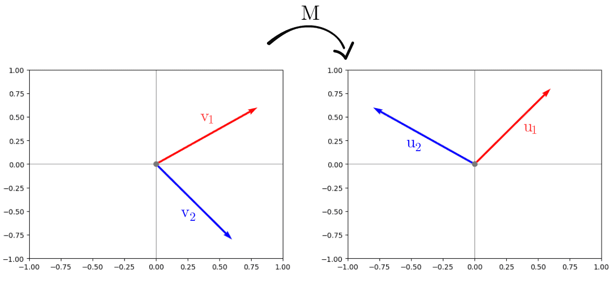
Since this is a fundamental concept in linear algebra, we’ll start with the orthogonality analysis. The columns of matrices $V$ and $U$ represent the set of orthogonal vectors that remains orthogonal after applying the transformation of matrix $M$ :

$M v_1 =\begin{bmatrix} 0.96 & 1.72 \\ 2.28 & 0.96 \end{bmatrix} \begin{bmatrix}0.8 \\ 0.6 \end{bmatrix} = \begin{bmatrix}0.6 \\ 0.8 \end{bmatrix} = u_1$

$M v_2 =\begin{bmatrix} 0.96 & 1.72 \\ 2.28 & 0.96 \end{bmatrix} \begin{bmatrix}0.6 \\ -0.8 \end{bmatrix} = \begin{bmatrix}-0.8 \\ 0.6 \end{bmatrix} = u_2$

We can easily verify the orthogonality before and after the transformation by plotting the vectors:

The second interpretation of the SVD is on an optimization problem. If we need to find out in which direction a matrix stretches a unit vector the most, we solve:

$argmax \lVert Ax \rVert \text{ subject to } \lVert x \rVert =1$

For the sake of simplicity, we won’t demonstrate here, but the solution for this problem is given by the first column of matrix $U$ ( $u_1$ ).

Now let’s see how SVD works on real-world applications.

4. Applications

We’ll discuss two different applications. First, we’ll show how SVD can compress an image then we’ll see how SVD can be used to analyze a high-dimensional dataset.

4.1. Image Compression

Considering that we proposed the model $M = U \Sigma V^{T}$ for the SVD, now let’s introduce the k-rank SVD model.

In this model, we’ll only consider the first $k$ columns of $U$ , the $k$ most significant singular values of $\Sigma$ , and the first $k$ rows of $V^{T}$ . To see this in practice, let’s consider a grayscale image of the Sagrada Familia Basilica in Barcelona for different low-rank approximations:

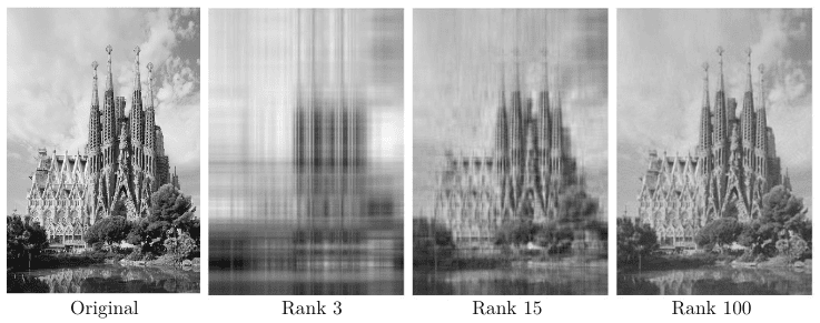
For a quantitative metric of compression, let’s consider the formula:

$\text{compression rate } = \frac{(\text{height } \times k) + k + (\text{width } \times k)}{\text{height} \times \text{width}}$

It is clear that for $k=3$ , we can barely see the church, but the compression rate is incredibly high, equal to 158. As we increase the rank to 15, our image becomes clearer. For that case, we have a compression rate of 31.79. Once we reach the highest rank in our experiments, the church is well represented, and our compression rate is equal to 4.76.

This illustrates the potential of the SVD in the image compression field, especially if we need to uncover essential features in an image.

As a final example, let’s discuss a second application of SVD called Principal Component Analysis (PCA).

4.2. PCA

A PCA aims to find linear combinations of the original coordinates of a matrix $M$ in the form:

$p_i = \sum_{j=1}^{n} w_{ij} m_{j}$

for $i=1, \ldots n$ . We’ll only highlight here that the components have to be orthogonal, which is the case of an SVD decomposition. For a more detailed description of PCA, we’ll refer to a previous article.

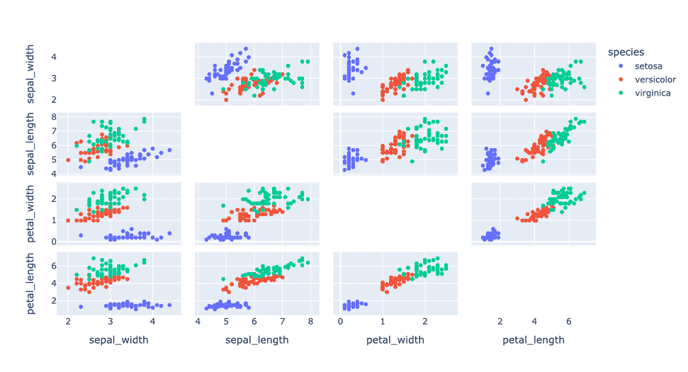
Here, we’ll see how the PCA can reduce dimensionality. We’ll use the traditional Iris dataset with four features: $sepal_width$ , $sepal_length$ , $petal_width$ , and $petal_length$ .

The complexity of the data is evidenced if we plot all the features in 2D for the three species of plants:

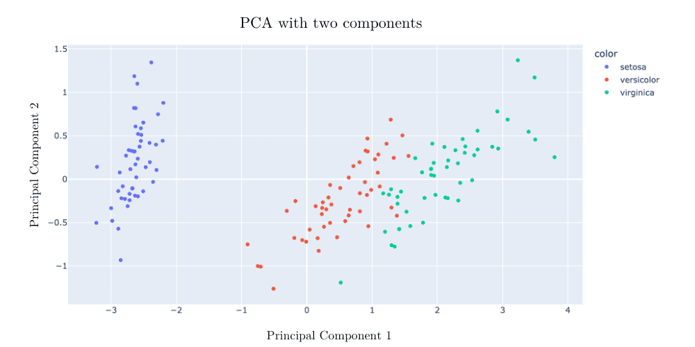
But once we perform a PCA with two components, the plants are successfully segmented:

5. Conclusion

In this article, we discussed the relevance and how to compute an SVD of a matrix. Many applications rely on the implementation of this method.

From insights and dimensionality reduction to linear algebra proofs, SVD plays a crucial role. We should keep in mind that after performing an SVD, we’ll end up with matrices that are easier to manipulate and have a strong interpretation, as we saw in this article.

Full Archive

About Baeldung

Core Concepts

Operating Systems

Artificial Intelligence

Graph Theory

Latex