

Learn through the super-clean Baeldung Pro experience:
>> Membership and Baeldung Pro.
No ads, dark-mode and 6 months free of IntelliJ Idea Ultimate to start with.
Learn through the super-clean Baeldung Pro experience:
>> Membership and Baeldung Pro.
No ads, dark-mode and 6 months free of IntelliJ Idea Ultimate to start with.
JPEG is one of the most widely-used picture formats on the internet.
In this tutorial, we’ll go through each step of the JPEG compression algorithm to learn how it works.
JPEG stands for Joint Photographic Experts Group and is a lossy compression algorithm that results in significantly smaller file sizes with little to no perceptible impact on picture quality and resolution. A JPEG-compressed image can be ten times smaller than the original one. JPEG works by removing information that is not easily visible to the human eye while keeping the information that the human eye is good at perceiving.
A lossy compression algorithm is a compression algorithm that permanently removes some data from the original file, especially redundant data, when compressing it. On the other hand, a lossless compression algorithm is a compression algorithm that doesn’t remove any information when compressing a file, and all information is restored after decompression.
First, let’s take a look at an overview of the steps that JPEG takes when compressing an image:
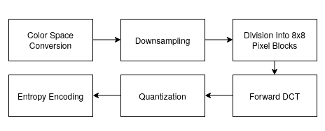
The above steps result in a .jpg image file.
A color space is a specific organization of colors. RGB (Red, Green, and Blue) and CMYK (Cyan, Magenta, Yellow, and Key/Black) are examples of color spaces. Moreover, each pixel in a picture has its color space values.
The human eye is more sensitive to brightness than color. Therefore, the algorithm can exploit this by making significant changes to the picture’s color information without affecting the picture’s perceived quality. To do this, JPEG must first change the picture’s color space from RGB to YCbCr.
YCbCr consists of 3 different channels: Y is the luminance channel containing brightness information, and Cb and Cr are chrominance blue and chrominance red channels containing color information. In this color space, JPEG can make changes to the chrominance channel to change the image’s color information without affecting the brightness information that is located in the luminance channel.
After conversion, each pixel has three new values that represent the luminance, the chrominance blue, and the chrominance red information.
After we separate the color information from the brightness information, JPEG downsamples the chrominance channels to a quarter of their original size. Each block of 4 pixels is averaged into a single color value for all 4 pixels. As a result, some information is lost, and the size of the picture is halved, but since the human eye is not very sensitive to color, the changes are not easily distinguishable.
It’s important to note that downsampling is only applied to the chrominance channels, and the luminance channel keeps its original size.
After downsampling, the pixel data of each channel is divided into 8×8 blocks of 64 pixels. From now on, the algorithm processes each block of pixels independently.
First, each pixel value for each channel is subtracted by 128 to make the value range from -128 to +127.
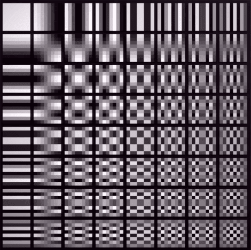
Using DCT, for each channel, each block of 64 pixels can be reconstructed by multiplying a constant set of base images by their corresponding weight values and then summing them up together. Here is what the base images look like:
Applying forward DCT on each block of 64 pixels gives us a matrix containing the corresponding weight values for each base image. These values show how much of each base image is used to reconstruct the original 8×8 pixel block, and it looks something like this:

For every block of 64 pixels, we’ll have three weight matrices, one for luminance and two for chrominance. In addition, no information is lost in this phase.
The human eye is not very good at perceiving high-frequency elements in an image. In this step, JPEG removes some of this high-frequency information without affecting the perceived quality of the image.
To do this, the weight matrix is divided by a precalculated quantization table, and the results are rounded to the closest integer. Here is what a quantization table for chrominance channels looks like:

And for the luminance channel:

We can see that the quantization tables have higher numbers at the bottom right, where high-frequency data is located, and have lower numbers at the top left, where low-frequency data is located. As a result, after dividing each weight value, high-frequency data is rounded to 0:

Now we have three matrices containing integer values for every block of 64 pixels, one for luminance and two for chrominance.
Now all that’s left to do is to list the values that are inside each matrix, run RLE (Run Length Encoding) since we have a lot of zeroes, and then run the Huffman Coding algorithm before storing the data.
RLE and Huffman Coding are lossless compression algorithms that reduce the space needed to store information without removing any data.
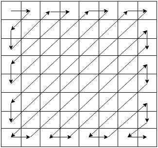
As we can see, the result of quantization has many 0s toward the bottom left corner. To keep the 0 redundancy, the JPEG algorithm does a zig-zag scanning pattern that keeps all zeroes together:
After zig-zag scanning, we get a list of integer values, and after running RLE on the list, we get each number and how many times they’re repeated.
Finally, JPEG runs Huffman coding on the result, and the values that have more frequency (like the zeroes) are represented with fewer bits than less frequent values.
No data is lost during this phase.
Whenever we open a .jpg file using an image viewer, the file needs to be decoded before it can be displayed. To decode a .jpg image, the image viewer does all the above steps in reverse order:
In this tutorial, we learned what happens when JPEG compresses image files and when an image viewer decodes a .jpg file to display on the screen.