How to Sort Mostly Sorted Arrays | Baeldung on Computer Science

1. Introduction

In this tutorial, we’ll analyze four standard sorting algorithms to see which one works best on mostly sorted input arrays.

2. Problem Statement

When it comes to sorting, we’re usually interested in the worst-case or the average-case complexity of an algorithm. Guided by the complexity analysis, we choose which algorithm to use.

However, the general-case analysis may not be suitable for the application at hand. When the input array is mostly sorted, that is, only a small percentage of its elements are out of the order, a poor-complexity algorithm may perform better than the theoretically superior one.

Here, we’ll analyze the performance of four sorting algorithms integer arrays that are already mostly sorted (in ascending order). We don’t lose generality that way because we can map the elements of an array to their integer indices. The only assumption is that, since the indices are unique, so too are the objects in the analyzed arrays. Therefore, our analysis won’t apply to the arrays with duplicates, but we can expect similar results for the arrays with a small number of repetitions.

3. Methodology

First, we have to define a mostly sorted array. Then, we’ll simulate such arrays and compare the performance of the selected sorting algorithms.

3.1. Mostly Sorted Arrays

We’ll say that an array $\boldsymbol{a = [a_1, a_2, \ldots, a_n]}$ is mostly sorted if only a small percentage of it is out of order. More precisely, such an array fulfills the following condition:

(1) $\begin{equation*} \alpha(a) = \frac{1}{n} \left\lvert \{ \{i, j\} \subset \{1,2,\ldots, n\} : i < j \land a_i > a_j\} \right\rvert \leq \varepsilon \end{equation*}$

where $\alpha(a)$ is the degree to which $a$ is mostly sorted, and $\varepsilon \in (0, 1)$ is the threshold for considering an array as such. Setting $\varepsilon$ to a small value like $0.01$ or $0.05$ , only the arrays with less than $1\%$ or $5\%$ unsorted elements fulfill the definition of “mostly sorted”.

We’ll call the pairs $(i, j)$ from Equation (1) inversions. As we’ll see, we can use several probabilistic models to construct an inversion, which is how we differentiate between different types of mostly sorted arrays.

3.2. Types of Mostly Sorted Arrays

We considered the following four types.

A left-perturbed array is the one that contains the inversions in its left part. In other words, the probability of an inversion drops exponentially from left to right. So, the inversions’ indices ( $k$ ) follow the geometric distribution with the CDF $1 - (1 - p)^k$ . To find $p$ , we impose the condition that $99\%$ of inversions should occur before the index that’s $\approx 20\% n$ :

$\begin{aligned} 1 - (1 - p)^{0.2n} &= 0.99 \\ (1 - p)^{0.2 n} &= 0.01 = 10^{-2}\\ 1- p &= 10^{-\frac{2}{0.2 n}} = 10^{-\frac{10}{n}} \\ p &= 1 - 10^{-\frac{10}{n}} \end{aligned}$

That’s not quite the actual distribution both indices follow in an inversion. The reason is that $j > i$ in an inversion $(i, j)$ . So, we use the above geometric distribution for the first index, $i$ , and draw $j$ repeatedly until we get a number different from $i$ . The same remark holds for the other types.

Analogously, a right-perturbed array contains the inversions in its right part. The corresponding distribution’s CDF is $1 -$ the CDF for left-perturbed arrays.

In centrally perturbed arrays, the inversions are around the middle element. Formally, we model the indices with the Gaussian distribution that contains $99.67\%$ of its mass between $[n/2 - n/10, n/2 + n/10]$ . So, the distribution’s mean is $n/2$ , and we get its standard deviation from the said condition:

$3\sigma &= \frac{n}{10} \\ \sigma &= \frac{n}{30} \implies \sigma^2 = \frac{n^2}{900}$

Finally, an inversion in a uniformly perturbed array can occur at any position. The corresponding distribution is uniform over $\{1,2,\ldots, n\}$ .

3.3. Algorithms

We analyzed four algorithms: Bubble Sort, Insertion Sort, Quicksort, and Merge Sort.

The first two were chosen because of the way they work. We suspected they’d perform well on our arrays. Merge Sort has a log-linear time complexity even in the worst case, which we wanted to verify empirically. Quicksort may be quadratic in the worst case but is $O(n \log n)$ in the average case, so we were interested in how it would handle our data.

3.4. Performance Metrics

The complexity of the sorting algorithms is usually expressed in terms of comparisons and swaps. For that reason, we implemented the algorithms to count both operations.

However, there isn’t a definitive rule which one is cheaper. If the objects are lightweight, such as floats, chars, or integers, we expect the swap to be the more expensive operation because it involves several steps. On the other hand, the objects may be very complex. So, comparing them could be a complex algorithm by itself. In those cases, it’s the number of comparisons that determines the complexity.

So, we consider both comparisons and swaps in our analysis. We also measured the execution time. However, those results aren’t set in stone. Different implementations on different hardware and operating systems may and probably will differ in running times.

4. Results

We’ll present the results separately for swaps, comparisons, and execution times (in seconds).

4.1. The Number of Swaps

All of the algorithms did more swaps as the input arrays contained more elements and inversions.

Here are the results of Bubble Sort:

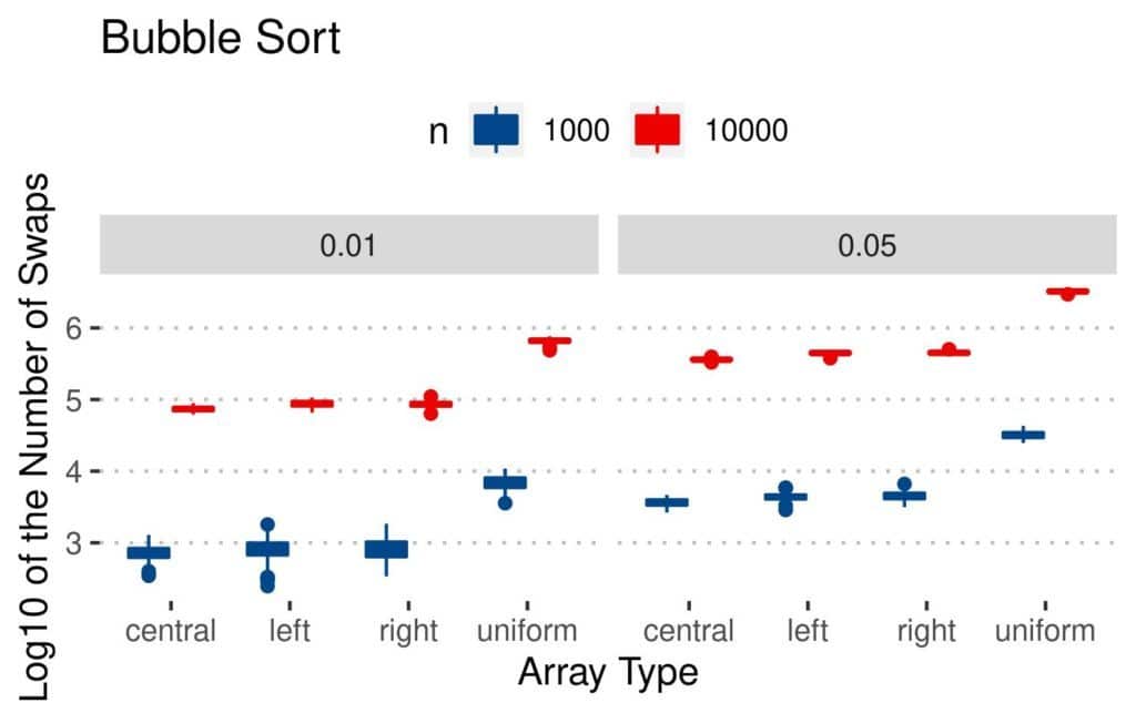
It does more swaps on uniformly perturbed arrays. A possible explanation is that the indices in uniform inversions are spread all over the array. The number of swaps in Bubble Sort depends primarily on the distances between the inverted elements. We expect them to be farther apart than the inverted indices in the other array types, where the inversions are concentrated in smaller parts of the arrays.

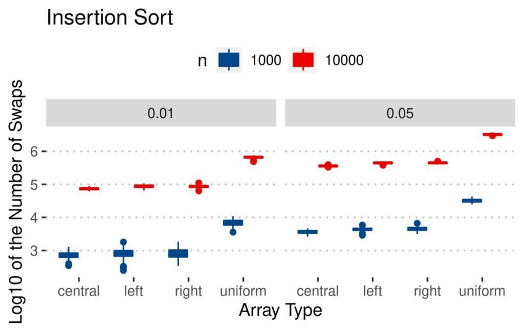
The results are similar for Insertion Sort:

On the other hand, the perturbation type doesn’t seem to affect the performance of Quicksort:

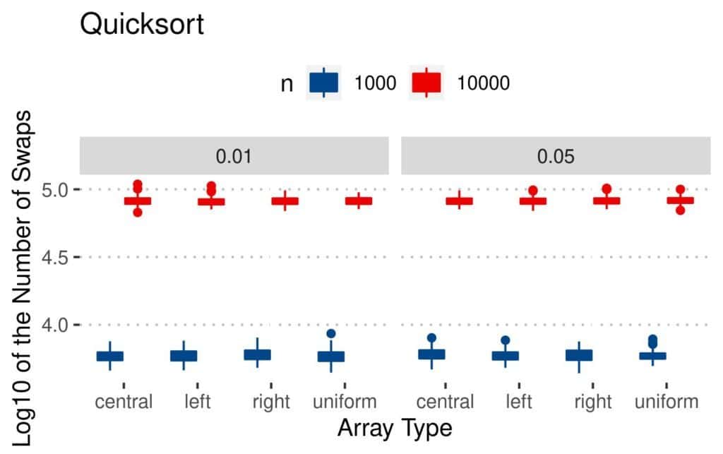
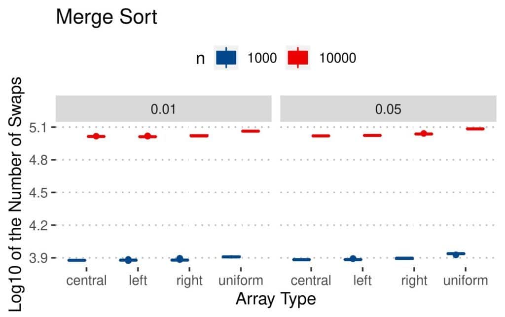
The reason is that its sorting logic is different. It does most of its work during partitioning. There, the number of swaps depends mainly on the selected pivots. Similar goes for Merge Sort:

Still, it seems that Bubble Sort and Insertion Sort did the fewest swaps on the arrays with $1000$ elements.

4.2. The Number of Comparisons

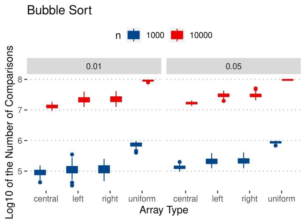
The conclusions are similar as for the number of swaps. As $n$ and $\varepsilon$ increased, so did the number of comparisons. However, Quicksort and Merge Sort appear stable across all the types, regardless of $\varepsilon$ . Bubble Sort and Insertion Sort performed worse on uniformly perturbed arrays. Overall, Insertion Sort looks like the best option when considering only the number of comparisons.

Let’s inspect the results of Bubble Sort:

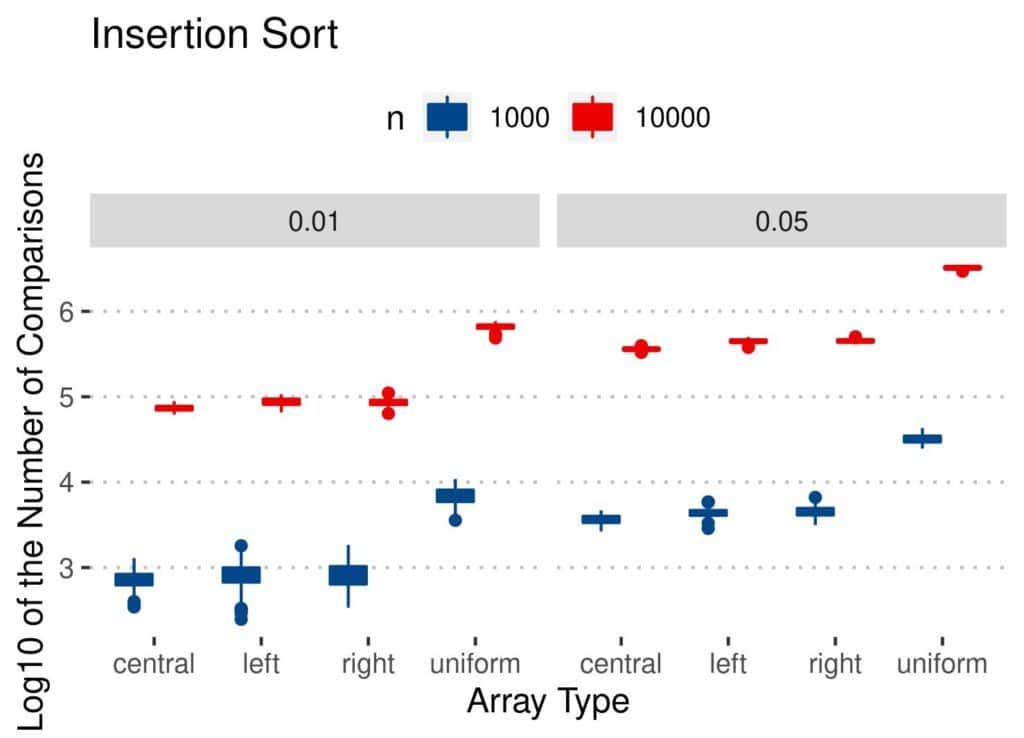
Insertion Sort has similar results:

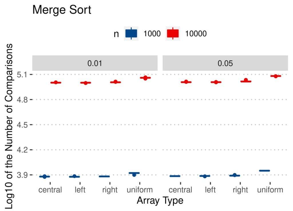
The results of Merge Sort are more or less the same as for the number of swaps:

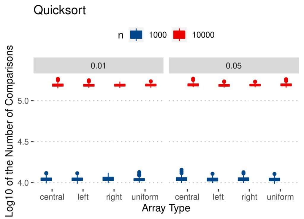
Finally, we can say the same for Quicksort:

4.3. The Execution Time

Let’s take a look at the execution time plots. Here’s how long Bubble Sort took to sort the arrays:

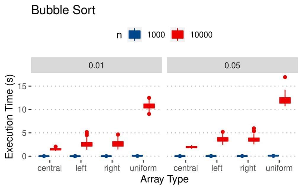
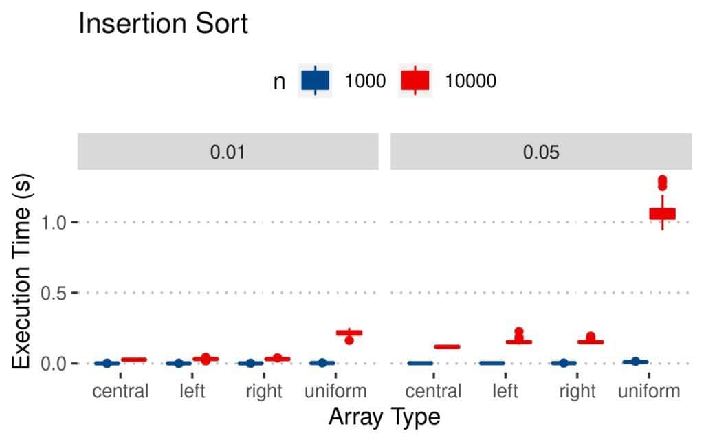
Uniformly perturbed arrays were more challenging than the other types. Conclusions are similar for Insertion Sort, except that it was faster:

Merge Sort was even faster, with more pronounced differences between the arrays with $1000$ and $10,000$ elements:

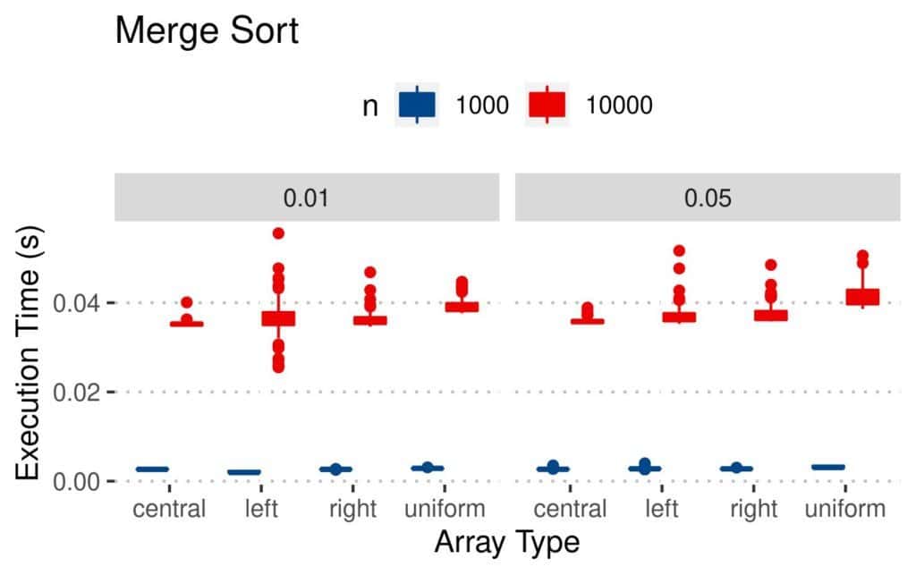
Quicksort behaved similarly to Merge Sort:

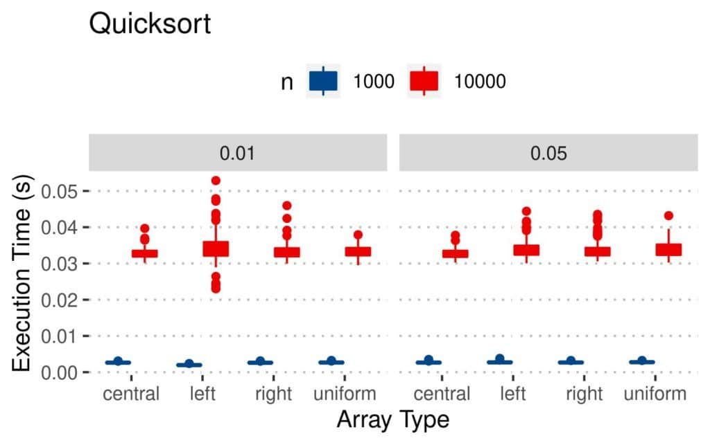
We may have been inclined to conclude that Insertion Sort is the optimal algorithm since it had consistently lower numbers of comparisons and swaps. However, as we see from the plots, the Quicksort and Merge Sort algorithms were the fastest.

Even though we may be reasonably confident in the accuracy of our results, we should note that the execution time doesn’t depend only on the algorithm run. The hardware and software environments, as well as the overhead caused by other programs being executed concurrently, may have affected the results.

5. Conclusion

In this tutorial, we talked about sorting the arrays that are already mostly sorted. We tested four standard sorting algorithms: Bubble Sort, Insertion Sort, Quicksort, and Merge Sort. To estimate their performance, we generated four types of mostly sorted arrays and counted the numbers of swaps and comparisons, as well as measured the execution time.

Overall, it seems that the Insertion Sort did the fewest swaps and comparisons in our experiment, but the fastest algorithms were Quicksort and Merge Sort. The results, therefore, confirm the theoretical analysis as Quicksort and Merge Sort has the best average-case time complexity, and the latter is optimal even in the worst case.

Still, since this was an empirical study, we should have in mind that replicating it with different arrays can give different results. That is the nature of empirical research.

Full Archive

About Baeldung

Core Concepts

Operating Systems

Artificial Intelligence

Graph Theory

Latex