Process Scheduling

1. Overview

In this tutorial, we’re going to explain how CPU scheduling works and we’ll clarify scheduling criteria and algorithms.

2. Definitions and Basic Concepts

The definition of a process is quite obvious, it’s the execution of a program or it’s simply a running program. However, to understand how it works we need to get into details about the operating system. Because the operating system makes processes live and makes them work. Other than that, the program just sits on the disk.

Imagine that, we’re writing an article about process scheduling, while we’re listening to music at the same time on our laptop or desktop. Also, there are hundreds of other browser tabs open. The system should allow all of these programs and they should run at the same time. Otherwise, we couldn’t run more than one program on our computers. While the OS handles this situation, it should let processes find a CPU is available.

At this point, we can think of that what if there is only one CPU, and there are more than hundreds of processes. The OS handles such issues by virtualizing the CPU. It can create the illusion of multiple CPUs by executing one process, then pausing it and starting another one, and so on. This fundamental concept, known as CPU time-sharing, enables users to run as many processes as they want.

Almost all modern OSes employ this time-sharing mechanism. Actually, the ability to stop one program and start another one on a given CPU is called, context switch. It has a crucial role in time-sharing and process scheduling.

2.1. Process States

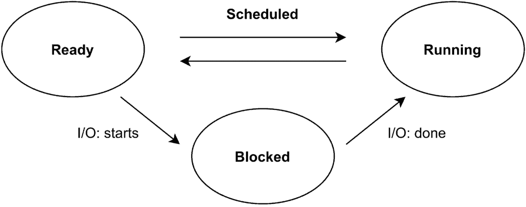
We’ve given a brief introduction about the definition of process and how the OS virtualizes the CPU in order to run more than one process concurrently. Now, we can look at the states of processes. There are simply three states in which a process can be:

• Running: In this state, a process is running on a processor and it’s executing its instructions.
• Ready: In the ready state, a process is ready to execute, but the operating system has decided not to launch it at this time for some reason.
• Blocked: In the blocked state, a process has completed some type of action that prevents it from running until another event occurs. As an example, when a process has an I/O request to a disk, it becomes blocked. This allows another process to access the CPU.

The figure below shows the transitions among process states:

3. Scheduling Criteria and Algorithms

Recently, people are encouraged to manage their time like schedulers in an OS. However, scheduling predates computer systems. Early techniques were adapted from the discipline of operations management and applied to computer systems. This is not a surprise that production lines and so many human efforts involve scheduling. Also, many of the same issues are valid for all of them.

In terms of CPU scheduling, there are some important metrics such as throughput, CPU utilization, turnaround time, waiting time, and response time. In the scope of this tutorial, we’re going to examine some scheduling algorithms in terms of turnaround time and response time.

Let’s give a piece of brief information about these important metrics:

• Turnaround time: It is the amount of time to execute a specific process. It actually equals to time at which the process completes minus the time at which the process arrives in the CPU.
• Response time: It is another important metric because turnaround time may not be sufficient on its own because of the processes that have long turnaround times. Response time represents the time from when the process arrives in a CPU to the first time it is scheduled.

3.1. First-In, First-Out (FIFO)

First In, First Out is one of the most basic algorithms that we can implement. While FIFO has some advantages such as it is clear and simple and so easy to implement, it has some drawbacks in such cases. It is also known as First-Come, First-Served (FCFS).

If we assume three processes arrive in the system, X, Y, and, Z. Let’s assume that the processes arrive in order X, Y, Z, and also each process runs for 20 seconds. The average turnaround time for  the three processes will be equal to the  seconds:

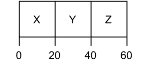
In this scenario, all of the processes have the same amount of execution time. What if they have different execution times. For example, what if X needs to run for 80 seconds while Y and Z run for 10 seconds. In that case, the turnaround time will be equal to   seconds.

We can see in the figure below why FIFO has some drawbacks as we mention in the earlier paragraphs. Y and Z processes have to wait until X is executed. This issue is generally known as the convoy effect:

3.2. Shortest-Job-First (SJF)

The name of this scheduling policy describes itself quite completely. It selects the shortest process first, and then the next shortest, it goes on like that:

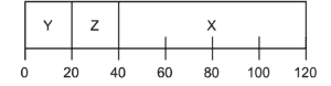
As we can see in the figure above, Y and Z don’t have to wait for X. SJF decreases average turnaround time, by running Y and Z before.  The average turnaround time equals to  seconds.

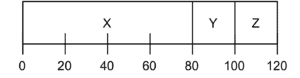
Even though SJF seems to work smoothly, in practical Y and Z don’t have to come at time 0, and time 20, respectively. What if X arrives at time 0 and needs to run for 80 seconds, and then, Y and Z arrive at time 20 as can we see in the figure below:

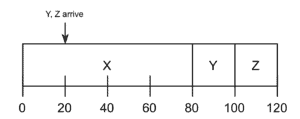
We go back to the same issue where Y and Z have to wait for the execution of X. This situation leads to the convoy problem again.  Average turnaround time is equal to seconds.

Also, if we consider the response time, we can see that SJF is not good for response time either. At this point, Round Robin comes into the stage, we’ll look at how it works in the next section.

3.3. Round Robin (RR)

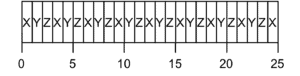
Rather than wait for the entire execution of a process, why not divide the time. We can split it into slices and change the process that we execute every time cycle as long as it is not completed. This is what RR policy does, and by doing that it reduces both average turnaround time and response time.  The average response time of RR is equal to second:

4. Conclusion

In this article, we’ve given brief information about the process and how they are scheduled in the CPU. We’ve also given an intuition about the scheduling criteria and algorithms.