

Learn through the super-clean Baeldung Pro experience:
>> Membership and Baeldung Pro.
No ads, dark-mode and 6 months free of IntelliJ Idea Ultimate to start with.
Last updated: August 30, 2024
Learn through the super-clean Baeldung Pro experience:
>> Membership and Baeldung Pro.
No ads, dark-mode and 6 months free of IntelliJ Idea Ultimate to start with.
In this tutorial, we’re going to look at the Quicksort algorithm and understand how it works.
Quicksort is a divide-and-conquer algorithm. This means that each iteration works by dividing the input into two parts and then sorting those, before combining them back together
It was originally developed by Tony Hoare and published in 1961 and it’s still one of the more efficient general-purpose sorting algorithms available.
The only real requirement for using the Quicksort algorithm is a well-defined operation to compare two elements. We can determine if any element is strictly less than another one. The exact nature of this comparison isn’t important, as long as it’s consistent. Note that direct equality comparison isn’t required, only a less-than comparison.
For many types, this is an undeniable comparison. For example, numbers implicitly define how to do this. Other types are less obvious, but we can still define this based on the requirements of the sort. For example, when sorting strings, we’d need to decide if a character case is important or how Unicode characters work.
The Binary Tree Sort is an algorithm where we build a balanced binary tree consisting of the elements we’re sorting. Once we have this, we can then build the results from this tree.
The idea is to select a pivot as a node on the tree, and then assign all elements to either the left or right branch of the node based on whether they are less than the pivot element or not. We can then recursively sort these branches until we have a completely sorted tree.
For example, to sort the list of numbers “3 7 8 5 2 1 9 5 4”, our first pass would be as follows:
Input: 3 7 8 5 2 1 9 5 4
Pivot = 3
Left = 2 1
Right = 7 8 5 9 5 4
This has given us two partitions from the original input. Everything in the Left list is strictly less than the Pivot, and everything else is in the Right list.
Next, we sort these two lists using the same algorithm:
Input: 2 1
Pivot = 2
Left = 1
Right = Empty

Input: 7 8 5 9 5 4
Pivot = 7
Left = 5 5 4
Right = 8 9
When we sorted the left partition from the first pass, we have ended up with two lists that have either length one or less. These are then already sorted – because it’s impossible to have a list of size one that is unsorted. This means that we can stop here, and instead focus on the remaining parts from the right partition.
At this point, we have the following structure:
      / [1]
    2
  /   \ []
3
  \   / [5 5 4]
    7
      \ [8 9]
We can see that we’re already getting close to a sorted list. We have two more partitions to sort, and then we’re finished:
        1
      /
    2       4
  /       /
3       5
  \   /   \
    7       5
      \
        8
          \
            9
This has sorted the list in 5 passes of the algorithm, applied to increasingly smaller sub-lists. However, the memory needs are relatively high, having had to allocate an additional 17 elements worth of memory to sort the nine elements in our original list.
Quicksort algorithm is similar in concept to a Binary Tree Sort. Rather than building sublists at each step that we then need to sort, it does everything in place within the original list.
It works by dynamically swapping elements within the list around a selected pivot, and by then recursively sorting the sub-lists to either side of this pivot. This makes it significantly more space-efficient, which can be important for huge lists.
Quicksort depends on two key factors — selecting the pivot and the mechanism for partitioning the elements.
The key to this algorithm is the partition function, which we’ll cover soon. This returns an index into the input array such that every element below this index sorts as less than the element at this index, and the element at this index sorts as less than all the elements above it.
Doing this will involve swapping some of the elements in the array around so that they are the appropriate side of this index.
Once we’ve done this partitioning, we then apply the algorithm to the two partitions on either side of this index. This eventually finishes when we have partitions that contain only one element each, at which point the input array is now sorted.
As a result, we can summarize the quick sort algorithm with three steps:
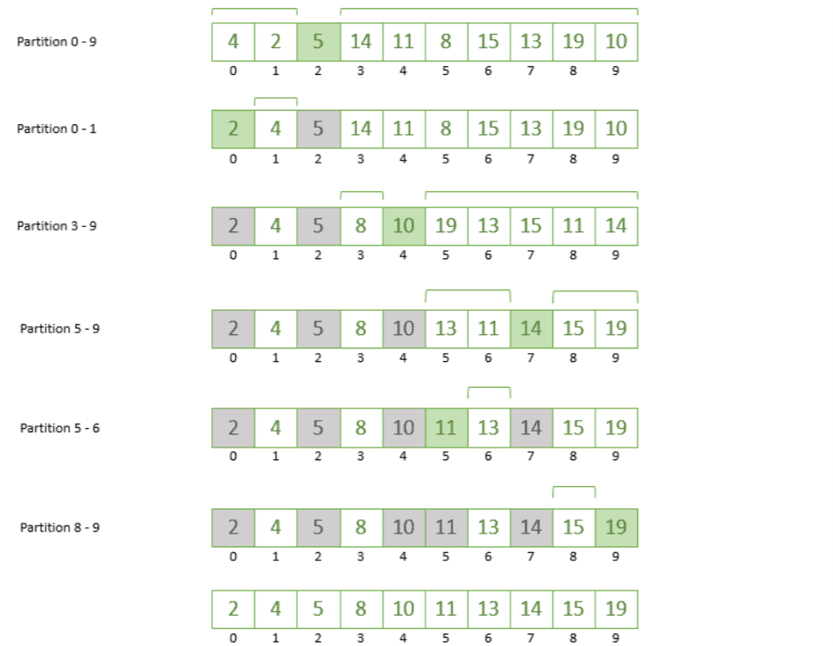
Here we have an array of ten unsorted values which we’re going to sort using Quicksort:
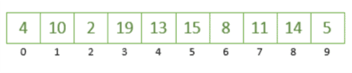
The first step we’re going to take is to choose an element from this array as our pivot. We can pick a pivot in different ways, but for this example, we’ll always pick the rightmost element of the array, which is the number 5.
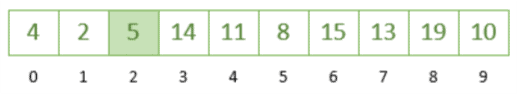
Now that we have determined 5 as our pivot, let’s partition the array based on our pivot by putting the numbers greater than 5 to the right and the numbers smaller than 5 to the left. At this point, we’re not really worried about ordering the numbers, just that we’ve moved them into the right place concerning the pivot.
In doing this, we’ve partitioned our array into two parts around the pivot 5:
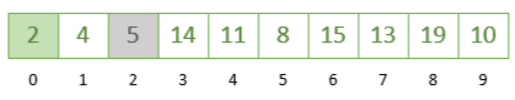
Let’s take the leftmost partition (index 0 – 1) and repeat the steps. We’re going to choose number 2 as our pivot and rearrange accordingly, which gives us the following:
Next, we take the rightmost partition (index 3 – 9) and take 10 as our pivot; any number greater than 10 will be moved to the right of it and the numbers smaller than 10 will go to its left:
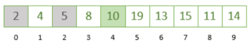
As we can see by positioning each chosen pivot, we’re slowly getting closer to a sorted array! If we continue repeating the steps on the remaining partition from index 5 to 9, we’ll finally reach a point where our array is sorted from smallest to largest.
The image below shows all the steps together finally giving us a sorted array:
As we can see, these steps can be different based on the way we choose the pivot element. Hence, let’s jump to discuss the main approaches to choosing the pivot.
The Quicksort algorithm has multiple implementations. These implementations differ from each other regarding the way of choosing the pivot element. Let’s discuss the partitioning methods.
Lomuto Partitioning is attributed to Nico Lomuto. This works by iterating over the input array, swapping elements that are strictly less than a pre-selected pivot element. They appear earlier in the array, but on a sliding target index.
This sliding target index is then the new partition index that we’ll return for the next recursions of the greater algorithm to work with.
This is to ensure that our sliding target index is in a position such that all elements before it in the array are less than this element and that this element is less than all elements after it in the array.
Let’s have a look at this in pseudocode:
fun quicksort(input : T[], low : int, high : int)
    if (low < high)
        p := partition(input, low, high)
        quicksort(input, low, p - 1)
        quicksort(input, p + 1, high)

fun partition(input: T[], low: int, high: int) : int
    pivot := input[high]
    partitionIndex := low
    loop j from low to (high - 1)
        if (input[j] < pivot) then
            swap(input[partitionIndex], input[j])
            partitionIndex := partitionIndex + 1
    swap(input[partitionIndex], input[high]
    return partitionIndex
As a worked example, we can partition our array from earlier:
Sorting input: 3,7,8,5,2,1,9,5,4 from 0 to 8
Pivot: 4
Partition Index: 0

When j == 0 => input[0] == 3 => Swap 3 for 3 => input := 3,7,8,5,2,1,9,5,4, partitionIndex := 1
When j == 1 => input[1] == 7 => No Change
When j == 2 => input[2] == 8 => No Change
When j == 3 => input[3] == 5 => No Change
When j == 4 => input[4] == 7 => Swap 7 for 2 => input := 3,2,8,5,7,1,9,5,4, partitionIndex := 2
When j == 5 => input[5] == 8 => Swap 8 for 1 => input := 3,2,1,5,7,8,9,5,4, partitionIndex := 3
When j == 6 => input[6] == 9 => No Change
When j == 7 => input[7] == 5 => No Change

After Loop => Swap 4 for 5 => input := 3,2,1,4,7,8,9,5,5, partitionIndex := 3
We can see from working through this that we have performed three swaps and determined a new partition point of index “3”. The array after these swaps is such that elements 0, 1, and 2 are all less than element 3, and element 3 is less than elements 4, 5, 6, 7, and 8.
Having done this, the greater algorithm then recurses, such that we’ll be sorting the sub-array from 0 to 2, and the sub-array from 4 to 8. For example, repeating this for the sub-array from 0 to 2, we will do:
Sorting input: 3,2,1,4,7,8,9,5,5 from 0 to 2
Pivot: 1
Partition Index: 0

When j == 0 => input[0] == 3 => No Change
When j == 1 => input[1] == 2 => No Change

After Loop => Swap 1 for 3 => input := 1,2,3,4,7,8,9,5,5, partitionIndex := 0
Note that we’re still passing the entire input array for the algorithm to work with, but because we’ve got low and high indices, we only actually pay attention to the bit we care about. This is an efficiency that means we’ve not needed to duplicate the entire array or sections of it.
Across the entire algorithm, sorting the entire array, we have performed 12 different swaps to get to the result.
Hoare partitioning was proposed by Tony Hoare when the Quicksort algorithm was originally published. Instead of working across the array from low to high, it iterates from both ends at once towards the center. This means that we have more iterations, and more comparisons, but fewer swaps.
This can be important since often comparing memory values is cheaper than swapping them.
In pseudocode:
fun quicksort(input : T[], low : int, high : int)
    if (low < high)
        p := partition(input, low, high)
        quicksort(input, low, p) // Note that this is different than when using Lomuto
        quicksort(input, p + 1, high)

fun partition(input : T[], low: int, high: int) : int
    pivotPoint := floor((high + low) / 2)
    pivot := input[pivotPoint]
    high++
    low--
    loop while True
        low++
        loop while (input[low] < pivot)
            high--
        loop while (input[high] > pivot)
        if (low >= high)
            return high
        swap(input[low], input[high])
As a worked example, we can partition our array from earlier:
Sorting input: 3,7,8,5,2,1,9,5,4 from 0 to 8
Pivot: 2

Loop #1
    Iterate low => input[0] == 3 => Stop, low == 0
    Iterate high => input[8] == 4 => high := 7
    Iterate high => input[7] == 5 => high := 6
    Iterate high => input[6] == 9 => high := 5
    Iterate high => input[5] == 1 => Stop, high == 5
    Swap 1 for 3 => input := 1,7,8,5,2,3,9,5,4
    Low := 1
    High := 4
Loop #2
    Iterate low => input[1] == 7 => Stop, low == 1
    Iterate high => input[4] == 2 => Stop, high == 4
    Swap 2 for 7 => input := 1,2,8,5,7,3,9,5,4
    Low := 2
    High := 3
Loop #3
    Iterate low => input[2] == 8 => Stop, low == 2
    Iterate high => input[3] == 5 => high := 2
    Iterate high => input[2] == 8 => high := 1
    Iterate high => input[1] == 2 => Stop, high == 1
    Return 1
On the face of it, this looks to be a more complicated algorithm that is doing more work. However, it does less expensive work overall. The entire algorithm only needs 8 swaps instead of the 12 needed by the Lomuto partitioning scheme to achieve the same results.
There are several adjustments that we can make to the normal algorithm, depending on the exact requirements. These don’t fit every single case, and so we should use them only when appropriate, but they can make a significant difference to the result.
The choice of the element to pivot around can be significant to how efficient the algorithm is. Above, we selected a fixed element. This works well if the list is truly shuffled in a random order, but the more ordered the list is, the less efficient this is.
If we were to sort the list 1, 2, 3, 4, 5, 6, 7, 8, 9 then the Hoare partitioning scheme does it with zero swaps, but the Lomuto scheme needs 44. Equally, the list 9, 8, 7, 6, 5, 4, 3, 2, 1 needs 4 swaps with Hoare and 24 with Lomuto.
In the Hoare partitioning scheme, this is already very good, but the Lomuto scheme can improve a lot. By introducing a change in how we select the pivot, by using a median of three fixed points, we can get a dramatic improvement.
This adjustment is known simply as Median-of-three:
mid := (low + high) / 2
if (input[mid] < input[low])
    swap(input[mid], input[low])
if (input[high] < input[low])
    swap(input[high], input[low])
if (input[mid] < input[high])
    swap(input[mid], input[high])
We apply this on every pass of the algorithm. This takes the three fixed points and ensures that they are pre-sorted in reverse order.
This seems unusual, but the impact speaks for itself. Using this to sort the list 1, 2, 3, 4, 5, 6, 7, 8, 9 now takes 16 swaps, where before it took 44. That’s a 64% reduction in the work done. However, the list 9, 8, 7, 6, 5, 4, 3, 2, 1 only drops to 19 swaps with this, instead of 24 before, and the list 3, 7, 8, 5, 2, 1, 9, 5, 4 goes up to 18 where it was 12 before.
Quicksort suffers slightly when there are large numbers of elements that are directly equal. It will still try to sort all of these, and potentially do a lot more work than is necessary.
One adjustment that we can make is to detect these equal elements as part of the partitioning phase and return bounds on either side of them instead of just a single point. We can then treat an entire stretch of equal elements as already sorted and just handle the ones on either side.
Let’s see this in pseudocode:
fun quicksort(input : T[], low : int, high : int)
    if (low < high)
        (left, right) := partition(input, low, high)
        quicksort(input, low, left - 1)
        quicksort(input, right + 1, high)
Every time the partitioning scheme returns a pivot, it returns the lower and upper indices for all adjacent elements that have the same value. This can quickly remove larger swaths of the list without needing to process them.
To implement this, we need to be able to compare elements for equality and less-than. However, this is typically an easier comparison to implement.
The Quicksort algorithm is generally considered to be very efficient. On average, it has  performance for sorting arbitrary inputs.
The original Lomuto partitioning scheme will degrade to  in the case where the list is already sorted and we pick the final element as the pivot. As we’ve seen, this improves when we implement median-of-three for our pivot selection, and in fact, this takes us back to
  .
.
Conversely, the Hoare partitioning scheme can result in more comparisons because it recurses on  instead of
  . This means the recursion makes more comparisons, even though it results in fewer swaps.
Here we’ve had an introduction to what Quicksort is and how the algorithm works. We’ve also covered some variations that can be made to the algorithm for different cases.