Sort Points in Clockwise Order | Baeldung on Computer Science

1. Introduction

Let’s imagine that we have a set of points on a $2D$ plane that we’d like to connect to draw a closed shape. First, we’d need to sort those points.

In our tutorial, we’re going to walk through a method that can sort $2D$ points in clockwise order.

2. Problem Explanation

Given a set of 2D points (each represented by $x$ and $y$ coordinates), we would like to sort these points in clockwise order. To begin, we need to view these points around a center point. This center-point can be at the $(0, 0)$ coordinates, or it could be at any arbitrary point on the 2D plane. Based on the requirements, we can choose which center point is better.

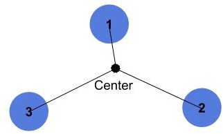
In our scenario, we’ll estimate the center point as the mean of the given points. This is shown in the following figure where we have 3 points sorted around the center point:

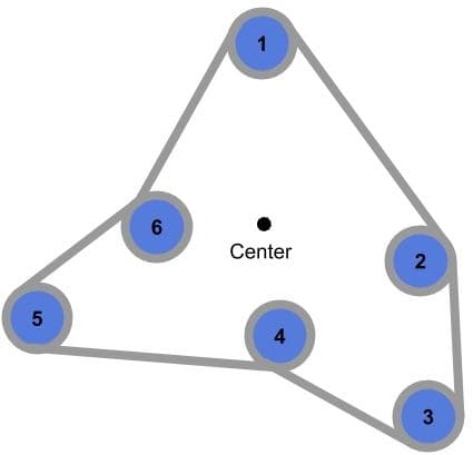
There are a few points to note here. First, we aren’t estimating the convex hull (the convex that encapsulates all points), but we’d like to find a closed path that goes through all the points in a clockwise order. Thus, it is fine to sort some points in the following way:

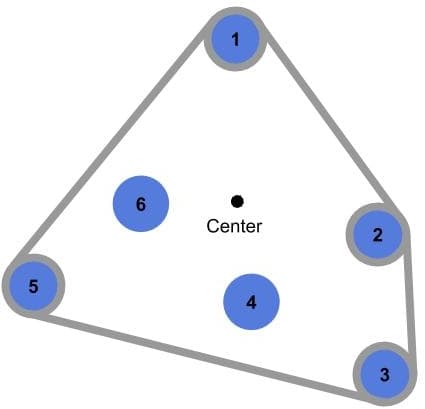
However, for the same set of points, if we estimate the convex hull, we’ll only include points 1, 2, 3, and 5 as follows:

One last thing to note is that we aren’t going to cover the exceptional case where all points lie on a straight line.

3. Algorithm Idea

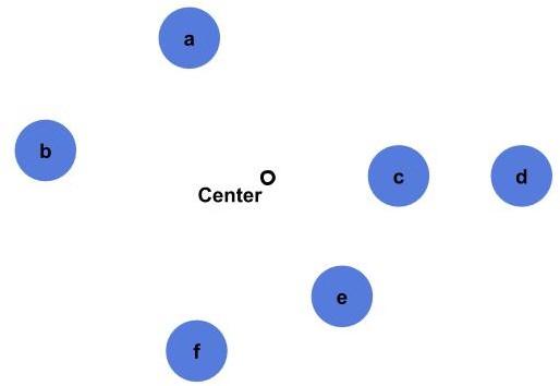
Let’s walk through an example given the set of points $a$ , $b$ , $c$ , $d$ , $e$ , and $f$ as shown:

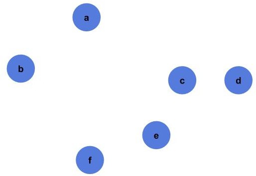
The first thing we need to do is to find the center point of the given points:

Then we estimate the angle between each point and the center:

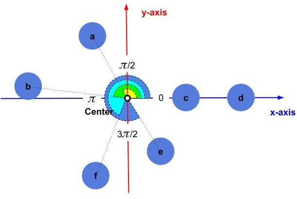
Since we need to sort the points in clockwise order, the first point will be point $e$ as it falls in the $4^{th}$ quadrant. Next will be point $f$ as it falls in the $3^{rd}$ quadrant. Points $b$ and $a$ are in the $2^{nd}$ quadrant; however, $b$ comes first as it is closer to $\pi$ , and $a$ is next. Finally, we have points $c$ and $d$ in the $1^{st}$ quadrant, but both are at angle $0^o$ . In this tutorial, we decided to break the tie by the distance from the center:

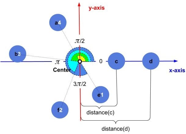
Since point $c$ is closer to the center than point $d$ , $c$ becomes the $5^{th}$ point, and $d$ is the last point in our order:

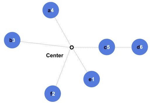
The final order in the given example will be $e$ , $f$ , $b$ , $a$ , $c$ , $d$ .

4. Flow-Chart

Now let’s see more details on how to design the algorithm.

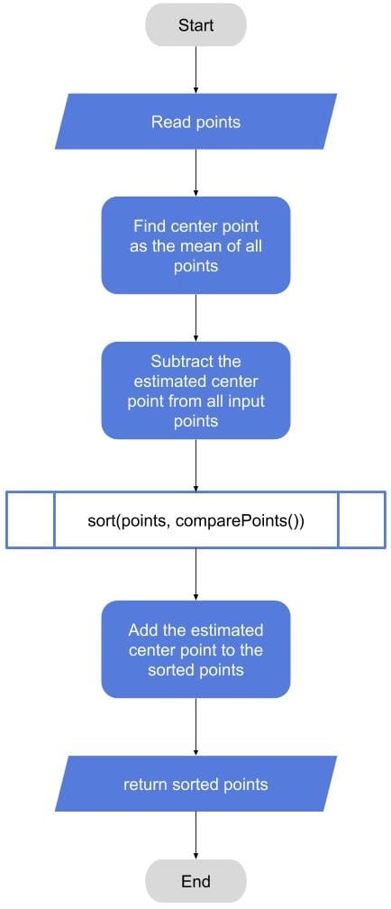
From a high-level perspective, we have an array of points that we need to sort according to some criteria. We can use any sorting algorithm and provide the right comparator to do the job; however, in our case, we need to add some pre- and post-processing steps.

For the pre-processing steps, we need to loop over the points to get the center point. Then we subtract this center point from all the given points so that we translate all the points to the new origin (center point).

Next, we call our sorting algorithm (like Quicksort or Bubble-Sort) with our $comparePoints$ function to get the points sorted according to our defined criteria. Finally, we re-add the center point to the sorted points to translate them back to the original location.

4.1. Sort Points Flow-Chart

Let’s start with the high-level idea illustrated in the following flow-chart:

4.2. Compare Points Flow-Chart

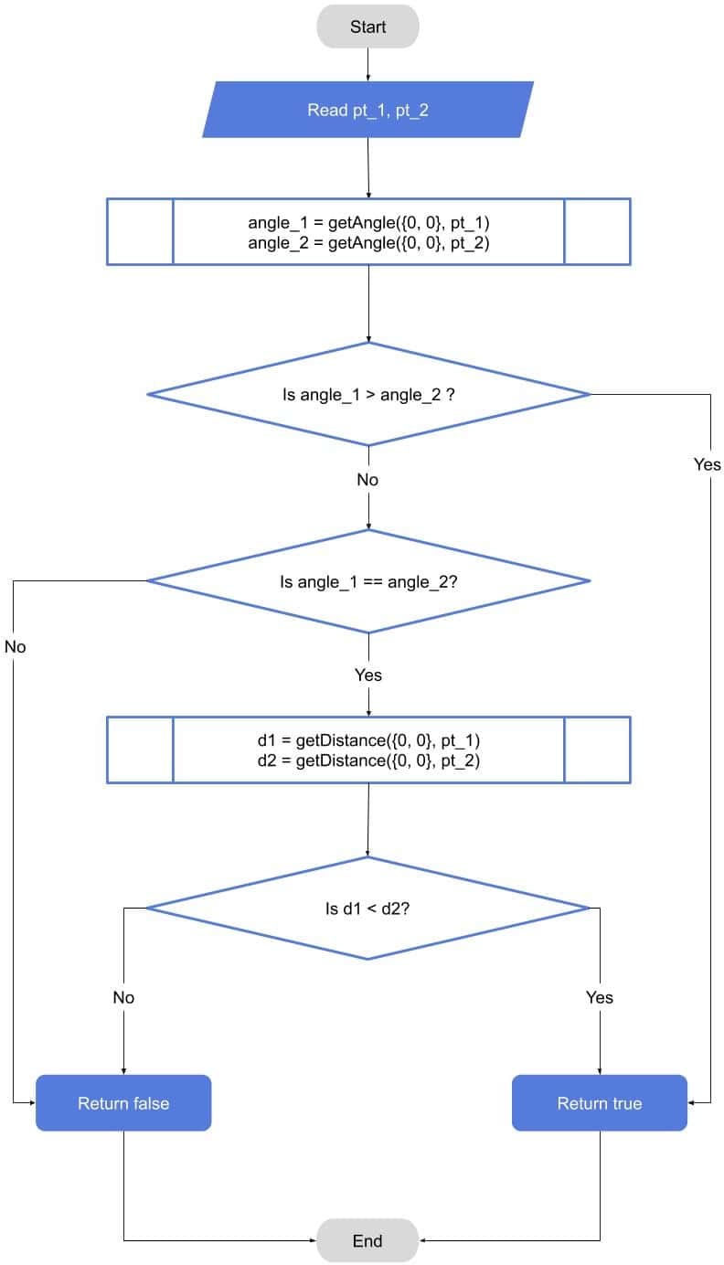
Now let’s dig deeper inside the $comparePoints$ function. In this function, we get two points as inputs, and we need to return $true$ if the first point comes before the second point, and $false$ otherwise. If we assume we have another function telling us the angle of any point relative to some center point from $0$ to $2\pi$ , then we can compare the two angles directly. In the case of a tie, we can compare the distance between each point and the center point, and then choose the smallest one.

The following flow-chart illustrates this idea. The center point is $\{0, 0\}$ because we translated all of our points around the center point in the pre-processing step:

The details for the $getAngle$ and $getDistance$ functions are going to be in the pseudocode.

5. Pseudocode

Now let’s look at simple pseudocode for our algorithm. The pseudocode starts with the general algorithm of finding the center point, and then translates all the points to this center. Next we call the sort function with our custom $comparePoints$ function. Finally, we move the sorted points back to the original locations:

algorithm sortPointsCW(Points):
    // INPUT
    //    Points = a set of 2D points
    // OUTPUT
    //    Points sorted in a clockwise order around their center

    pt_center <- (0, 0)
    for pt in Points:
        pt_center.x <- pt_center.x + pt.x
        pt_center.y <- pt_center.y + pt.y

    n <- the number of points in Points

    pt_center.x <- pt_center.x / n
    pt_center.y <- pt_center.y / n

    for pt in Points:
        pt.x <- pt.x - pt_center.x
        pt.y <- pt.y - pt_center.y

    sort Points using function comparePoints for comparison

    for pt in Points:
        pt.x <- pt.x + pt_center.x
        pt.y <- pt.y + pt_center.y

    return Points

Our $comparePoints$ function then calls the $getAngle$ and $getDistance$ functions for each pair of points. The function returns $true$ in the cases where the first angle is bigger than the second angle. In the cases where the angles are equal, or the first distance is less than the second distance:

function comparePoints(pt_center, pt_1, pt_2):
    // INPUT
    //    pt_center = the center point around which to sort
    //    pt_1, pt_2 = points to compare
    // OUTPUT
    //    Returns true if pt_1 comes before pt_2 in the clockwise order

    angle_1 <- getAngle((0,0), pt_1)
    angle_2 <- getAngle((0,0), pt_2)
    if angle_1 < angle_2:
        return true

    d1 <- getDistance((0,0), pt_1)
    d2 <- getDistance((0,0), pt_2)

    if (angle_1 = angle_2) and (d1 < d2):
        return true

    return false

Now let’s see how to estimate the angle. We’re going to assume that we’re using a function like $atan2$ that exists in many programming languages. This function estimates the angle using inverse tan based on the value of $y$ and $x$ , and returns the result in the range $-\pi$ to $\pi$ . In our case, we need the angle to be between $0$ and $2\pi$ . One way to do this is if the angle is less than $0$ , we add $2\pi$ . Thus, the final value of the angle will be in the desired range from $0$ to $2\pi$ :

function getAngle(pt_center, pt):
    // INPUT
    //    pt_center = the center point from which to measure the angle
    //    pt = the point whose angle is being measured
    // OUTPUT
    //    the angle (from 0 to 2*PI) of pt relative to pt_center

    x <- pt.x - pt_center.x
    y <- pt.y - pt_center.y

    angle <- atan2(y, x)

    if angle <= 0:
        angle <- 2 * PI + angle

    return angle

As for the distance, we can use simple Euclidean distance as the square root ( $sqrt$ ) of the sum of the square of the differences for all axes. In practice, we can get rid of the square root step and return the squared distance (in our scenario the distance is always between some point and the center point):

function getDistance(pt_1, pt_2):
    // INPUT
    //    pt_1, pt_2 = the points between which to calculate the distance
    // OUTPUT
    //    the Euclidean distance between pt_1 and pt_2
    
    x <- pt_1.x - pt_2.x
    y <- pt_1.y - pt_2.y
    
    return sqrt(x * x + y * y)

Please note that the sorting algorithm itself is out of the scope of this tutorial. We can use any available sorting algorithm like Quicksort to get a complexity of $O(n\: log(n))$ .

6. Complexity

The time complexity of our algorithm is the complexity of the selected sorting algorithm. If we choose Quicksort, the overall algorithm complexity will be $O(n\: log(n))$ . The reason is that we only have loops of complexity $O(n)$ for pre- and post-processing. Then we call the sorting algorithm with our custom compare function.

As for the space complexity, the algorithm doesn’t need to store any information apart from the center point. Therefore, the space complexity is $O(1)$ .

7. Conclusion

In this article, we presented a method to sort points in clockwise order. The idea depends on any general sorting algorithm with some pre- and post-processing steps. We illustrated the algorithm through an example, flow-charts, and pseudocode. Finally, we provided a simple complexity analysis of space and time complexities for the presented method.

Full Archive

About Baeldung

Core Concepts

Operating Systems

Artificial Intelligence

Graph Theory

Latex