Euclidean Distance vs Cosine Similarity | Baeldung on Computer Science

1. Overview

In this tutorial, we’ll study two important measures of distance between points in vector spaces: the Euclidean distance and the cosine similarity.

We’ll then see how can we use them to extract insights on the features of a sample dataset. We’ll also see when should we prefer using one over the other, and what are the advantages that each of them carries.

2. Measuring Distances in Vector Spaces

2.1. What Is Distance?

Both cosine similarity and Euclidean distance are methods for measuring the proximity between vectors in a vector space. It’s important that we, therefore, define what do we mean by the distance between two vectors, because as we’ll soon see this isn’t exactly obvious.

Let’s start by studying the case described in this image:

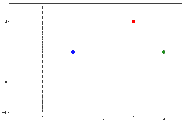
We have a 2D vector space in which three distinct points are located: blue, red, and green. We could ask ourselves the question as to which pair or pairs of points are closer to one another. As we do so, we expect the answer to be comprised of a unique set of pair or pairs of points:

If only one pair is the closest, then the answer can be either (blue, red), (blue, green), or (red, green)
If two pairs are the closest, the number of possible sets is three, corresponding to all two-element combinations of the three pairs
Finally, if all three pairs are equally close, there is only one possible set that contains them all

This means that the set with the closest pair or pairs of points is one of seven possible sets. How do we determine then which of the seven possible answers is the right one? To do so, we need to first determine a method for measuring distances.

2.2. Measuring Distances With Rulers

We can determine which answer is correct by taking a ruler, placing it between two points, and measuring the reading:

If we do this for all possible pairs, we can develop a list of measurements for pair-wise distances. By sorting the table in ascending order, we can then find the pairwise combination of points with the shortest distances:

In this example, the set comprised of the pair (red, green) is the one with the shortest distance. We can thus declare that the shortest Euclidean distance between the points in our set is the one between the red and green points, as measured by a ruler.

2.3. Measuring Distances With Goniometers

We can also use a completely different, but equally valid, approach to measure distances between the same points.

Let’s imagine we are looking at the points not from the top of the plane or from bird-view; but rather from inside the plane, and specifically from its origin. If we do this, we can represent with an arrow the orientation we assume when looking at each point:

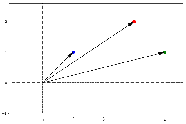
From our perspective on the origin, it doesn’t really matter how far from the origin the points are. In fact, we have no way to understand that without stepping out of the plane and into the third dimension.

As far as we can tell by looking at them from the origin, all points lie on the same horizon, and they only differ according to their direction against a reference axis:

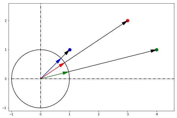
We really don’t know how long it’d take us to reach any of those points by walking straight towards them from the origin, so we know nothing about their depth in our field of view. What we do know, however, is how much we need to rotate in order to look straight at each of them if we start from a reference axis:

We can at this point make a list containing the rotations from the reference axis associated with each point. We can subsequently calculate the distance from each point as a difference between these rotations. If we do so we obtain the following pair-wise angular distances:

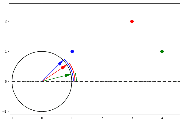
We can notice how the pair of points that are the closest to one another is (blue, red) and not (red, green), as in the previous example. We can in this case say that the pair of points blue and red is the one with the smallest angular distance between them.

Note how the answer we obtain differs from the previous one, and how the change in perspective is the reason why we changed our approach.

2.4. The Generalization to Higher Dimensions

What we’ve just seen is an explanation in practical terms as to what we mean when we talk about Euclidean distances and angular distances.

In the example above, Euclidean distances are represented by the measurement of distances by a ruler from a bird-view while angular distances are represented by the measurement of differences in rotations.

Let’s now generalize these considerations to vector spaces of any dimensionality, not just to 2D planes and vectors.

3. A Formal Definition of Euclidean Distance

In ℝ $^n$ , the Euclidean distance $||x-y||_2$ between two vectors $x = (x_1, x_2, ..., x_n)$ and $y = (y_1, y_2, ... , y_n)$ is always defined. It corresponds to the L2-norm $||.||_2$ of the difference $x-y$ between the two vectors. It can be computed as:

$||x-y||_2 = \sqrt{\sum_{i=1}^{n}{(x_i-y_i)^2}} = \sqrt{(x_1-y_1)^2+(x_2-y_2)^2+...+(x_n-y_n)^2}$

A vector space where Euclidean distances can be measured, such as $\mathbb{R}^n$ , $\mathbb{C}^n$ , $\mathbb{Z}^n$ , is called a Euclidean vector space.

Most vector spaces in machine learning belong to this category.

This means that when we conduct machine learning tasks, we can usually try to measure Euclidean distances in a dataset during preliminary data analysis. Some machine learning algorithms, such as K-Means, work specifically on the Euclidean distances between vectors, so we’re forced to use that metric if we need them.

4. A Formal Definition of Cosine Similarity

If we go back to the example discussed above, we can start from the intuitive understanding of angular distances in order to develop a formal definition of cosine similarity.

Cosine similarity between two vectors corresponds to their dot product divided by the product of their magnitudes. If $x$ and $y$ are vectors as defined above, their cosine similarity $cos(\theta)$ is:

$cos(\theta) = \frac{x \cdot y}{||x|| \cdot ||y||}$

The relationship between cosine similarity and the angular distance which we discussed above is fixed, and it’s possible to convert from one to the other with a formula:

$Ang. dist. = \frac{cos^{-1}(cos(\theta))}{\pi}$

5. Euclidean Distance and Cosine Similarity in the Iris Dataset

5.1. Clusterization Based on Euclidean Distances

Let’s take a look at the famous Iris dataset, and see how can we use Euclidean distances to gather insights on its structure. This is its distribution on a 2D plane, where each color represents one type of flower and the two dimensions indicate length and width of the petals:

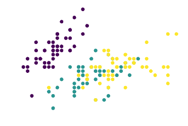
We can use the K-Means algorithm to cluster the dataset into three groups.

The K-Means algorithm tries to find the cluster centroids whose position minimizes the Euclidean distance with the most points. In red, we can see the position of the centroids identified by K-Means for the three clusters:

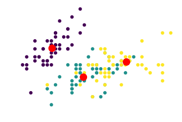
Clusterization of the Iris dataset on the basis of the Euclidean distance shows that the two clusters closest to one another are the purple and the teal clusters. We’re going to interpret this statement shortly; let’s keep this in mind for now while reading the next section.

5.2. Clusterization Based on Cosine Similarity

As we have done before, we can now perform clusterization of the Iris dataset on the basis of the angular distance (or rather, cosine similarity) between observations.

Remember what we said about angular distances: We imagine that all observations are projected onto a horizon and that they are all equally distant from us. The picture below thus shows the clusterization of Iris, projected onto the unitary circle, according to spherical K-Means:

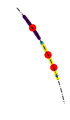
We can see how the result obtained differs from the one found earlier.

It appears this time that teal and yellow are the two clusters whose centroids are closest to one another. This is because we are now measuring cosine similarities rather than Euclidean distances, and the directions of the teal and yellow vectors generally lie closer to one another than those of purple vectors.

This answer is consistent across different random initializations of the clustering algorithm and shows a difference in the distribution of Euclidean distances vis-à-vis cosine similarities in the Iris dataset.

5.3. Interpreting the Clusterizations Over the Iris Dataset

We can now compare and interpret the results obtained in the two cases in order to extract some insights into the underlying phenomena that they describe:

Clusterization according to Euclidean distance tells us that purple and teal flowers are generally closer to one another than yellow flowers. This means that the sum of length and width of petals, and therefore their surface areas, should generally be closer between purple and teal than between yellow flowers and any others
Clusterization according to cosine similarity tells us that the ratio of features, width and length, is generally closer between teal and yellow flowers than between yellow and any others. This tells us that teal and yellow flowers look like a scaled-up version of the other, while purple flowers have a different shape altogether

The interpretation that we have given is specific for the Iris dataset. Its underlying intuition can however be generalized to any datasets. Vectors whose Euclidean distance is small have a similar “richness” to them; while vectors whose cosine similarity is high look like scaled-up versions of one another.

6. When Should We Prefer One Over the Other?

The decision as to which metric to use depends on the particular task that we have to perform:

Some tasks, such as preliminary data analysis, benefit from both metrics; each of them allows the extraction of different insights on the structure of the data
Others, such as text classification, generally function better under Euclidean distances
Some more, such as retrieval of the most similar texts to a given document, generally function better with cosine similarity

As is often the case in machine learning, the trick consists in knowing all techniques and learning the heuristics associated with their application. This is acquired via trial and error.

The way to speed up this process, though, is by holding in mind the visual images we presented here. If we do so, we’ll have an intuitive understanding of the underlying phenomenon and simplify our efforts.

7. Conclusions

In this article, we’ve studied the formal definitions of Euclidean distance and cosine similarity. The Euclidean distance corresponds to the L2-norm of a difference between vectors. The cosine similarity is proportional to the dot product of two vectors and inversely proportional to the product of their magnitudes.

We’ve also seen what insights can be extracted by using Euclidean distance and cosine similarity to analyze a dataset. Vectors with a small Euclidean distance from one another are located in the same region of a vector space. Vectors with a high cosine similarity are located in the same general direction from the origin.

Full Archive

About Baeldung

Core Concepts

Operating Systems

Artificial Intelligence

Graph Theory

Latex