

Learn through the super-clean Baeldung Pro experience:
>> Membership and Baeldung Pro.
No ads, dark-mode and 6 months free of IntelliJ Idea Ultimate to start with.
Learn through the super-clean Baeldung Pro experience:
>> Membership and Baeldung Pro.
No ads, dark-mode and 6 months free of IntelliJ Idea Ultimate to start with.
The mean, variance, mode, and median of a dataset are the most common statistical quantities we use in many different fields of engineering, data science, and social sciences. However, we may sometimes need to go beyond these quantities as they give a limited idea about the shape of a probability distribution.
Skewness and kurtosis are statistical quantities that might give a better idea about the shape of a distribution.
In this tutorial, we’ll discuss skewness and kurtosis in statistics. Firstly, we’ll discuss the definitions of them together with a more general concept, namely moments. Then, we’ll see several examples of distributions with different skewness and kurtosis values. Finally, we’ll discuss a few applications of them in different fields.
We’ll discuss the definitions of skewness and kurtosis in this section. They’re special cases of moments.
Moments of a random variable describe several aspects of the shape of its probability density function.
Let’s suppose X is a discrete random variable, and r is a non-negative integer. In that case, we can calculate the rth moment of X using the probability density function of X, namely f(x):
![E[X^r]=\sum_{x} x^rf(x)](/wp-content/ql-cache/quicklatex.com-0766f78947b3a291238b91a02d4866ce_l3.svg "Rendered by QuickLaTeX.com")
This definition of the moment is also known as the raw moment. E[X] denotes the expected value of X. There are other variations of moments, i.e., central moments and standardized moments.
We can write the rth central moment of X using the probability density function of X as:
![E[(X -\mu)^r]=\sum_{x} (x -\mu)^rf(x)](/wp-content/ql-cache/quicklatex.com-bfc4d8fe3414c81f751dfb28401265fe_l3.svg "Rendered by QuickLaTeX.com")
It’s possible to normalize a central moment by dividing it with a power of the standard deviation. We can write the normalized rth central moment of X as:
![\dfrac{E[(X -\mu)^r]}{\sigma^r}](/wp-content/ql-cache/quicklatex.com-54de96a8fca523a85cfec2f2321ba734_l3.svg "Rendered by QuickLaTeX.com")
 is the standard deviation. The normalized rth central moment is also known as the standardized moment. Standardized moments are dimensionless because of the division.
The mean and variance are special cases of moments. The mean of a random variable X, which is the average of the samples in a dataset, is the first raw moment. The variance, which measures the dispersion of the samples of a distribution from the mean, is the second central moment of X.
Although the mean and variance are among the most widely used statistical quantities, two datasets having the same mean and variance may have different distributions. Therefore, we may sometimes need to go beyond the second-order moments of a distribution.
Skewness is a measure of the asymmetry of a distribution around its mean. It’s the normalized third-order central moment of a random variable X:
![\dfrac{E[(X -\mu)^3]}{\sigma^3}](/wp-content/ql-cache/quicklatex.com-3e6e4a98d2cb81b22695cd6741fc6ebf_l3.svg "Rendered by QuickLaTeX.com")
The skewness of a symmetrical distribution around its mean is 0. However, asymmetrical distributions can have positive or negative skewness values.
An unimodal distribution with a positive skewness has its mean on the left part of the distribution. An unimodal distribution is a distribution having a single peak.
Distributions with a positive skewness have a longer right tail. So, they’re named as right-skewed or right-tailed. Generally, for a distribution with positive skewness, the mean of the distribution is greater than its median, and the median is greater than its mode. They’re generally close to each other for a symmetrical distribution.
On the contrary, if a distribution has a negative skewness, then the left tail is longer. A unimodal distribution with a negative skewness has its mean on the right part of the distribution. Therefore, they’re named as left-skewed or left-tailed. Generally, for a distribution with a negative skewness, the mean of the distribution is less than its median, and the median is less than its mode.
Kurtosis is a measure of the dispersion of a distribution between its peak and tails. It’s the normalized fourth-order central moment of a random variable X:
![\dfrac{E[(X -\mu)^4]}{\sigma^4}](/wp-content/ql-cache/quicklatex.com-f0f6d904d7bbb3a298cc4a41d1ac4ae9_l3.svg "Rendered by QuickLaTeX.com")
Kurtosis measures the curvature of the tails of a distribution. The kurtosis of the normal distribution is 3. Distributions having a kurtosis value close to 3 are named mesokurtic or mesokurtotic distributions. Meso means middle in ancient Greek.
Distributions having a kurtosis value greater than 3 are leptokurtic or leptokurtotic distributions. Lepto means slender in ancient Greek. There’s a greater tendency in the number of outliers for a leptokurtic distribution i.e., it has fatter tails.
The Rayleigh distribution and Poisson distribution are examples of leptokurtic distributions.
Distributions having a kurtosis value less than 3 are platykurtic or platykurtotic distributions. Platy means flat in ancient Greek. Platykurtic distributions have thinner tails, i.e., they have fewer outliers.
The uniform distribution and Bernoulli distribution with p=1/2 are typical examples of platykurtic distributions.
It’s a common practice to use the excess kurtosis instead of kurtosis. We calculate the excess kurtosis by subtracting 3 from kurtosis, i.e., the excess kurtosis measures how heavily the tails of a distribution differ from the tails of the normal distribution. Therefore, a distribution with positive excess kurtosis is leptokurtic while a distribution with negative excess kurtosis is platykurtic. On the other hand, a distribution having an excess kurtosis value of 0 is mesokurtic.
In this section, we’ll examine several distributions having different values of skewness and kurtosis.
Let’s consider the dataset below:
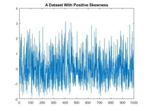
This dataset consists of 1000 samples. Its mean is 0 and variance is 1. However, the samples aren’t evenly distributed around the mean. This becomes evident if we plot the histogram of the dataset:
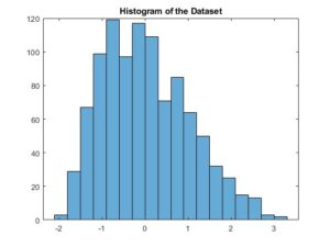
Apparently, the mass of the distribution is concentrated on the left part of the histogram, i.e., the distribution seems to be leaning to the left. The skewness of the dataset is approximately 0.6.
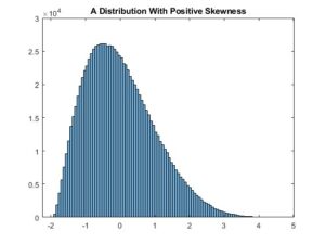
If we plot the histogram using a larger dataset with 1000000 samples, we obtain a smoother histogram. The mean of this distribution is 0, its variance is 1, and its skewness is 0.6:
Below is the histogram of a dataset having 1000000 samples with mean 0, variance 1, and skewness -0.6:
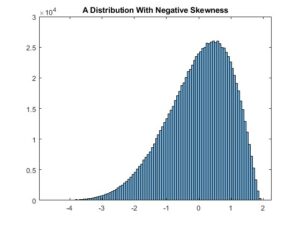
As is apparent from the histogram above, the mass of a distribution with a negative skewness is concentrated on the right part of the histogram, i.e., the distribution seems to be leaning to the right.
Let’s consider the following leptokurtic distribution:
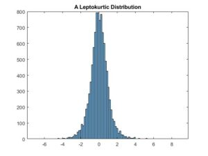
The mean, variance, and skewness of this distribution are 0, 1, and 0, respectively. The kurtosis of the distribution is 10. As is apparent from the histogram, the values of the dataset’s samples are approximately between -8 and 10. It has a sharp peak around 0, as expected.
The following platykurtic distribution has a kurtosis value of 2.5:
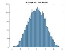
The mean, variance, and skewness of this distribution are also 0, 1, and 0, respectively. In this case, the values of the dataset’s samples are approximately between -3 and 3. Apparently, this distribution has a smaller number of outliers than the previous distribution. The peak is broader in this case, as expected.
Finally, let’s have a look at a mesokurtic distribution with zero skewness:
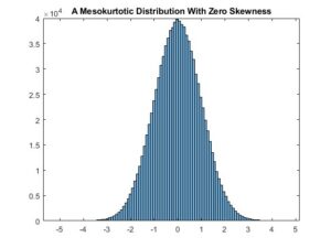
The mean and variance of this distribution are 0 and 1, respectively, like the previous distributions.
Skewness and kurtosis play an important role in many different fields since analyzing datasets using only mean and variance may not always be sufficient.
For example, with increasing life expectancy and declining birth rates, the age distribution in some countries is left-skewed. This implies an aging population. A left-skewed age distribution may encourage governments of those countries to take precautions to increase the population growth rate.
On the contrary, some countries have a right-skewed age distribution. An increasing population might have several effects in the future, such as increasing employment and environmental problems. So, the governments of those countries may make plans to decrease the population growth rate.
As the distribution of income in a country becomes more leptokurtic, the number of very rich and very poor people increases. This might be an indication of income inequality.
Investors in a stock market should consider the income statistics of assets. For example, a risk lover may invest in more leptokurtic assets, while a cautious investor may invest in more platykurtic assets to mitigate risks.
Skewness and kurtosis find usage also in digital signal processing, for instance in blind equalization of fading channels.
Traditionally, the equalization of fading channels is accomplished by either sending training sequences before the communication or by designing an equalizer based on a priori knowledge of the channel. However, it’s possible to estimate the transmitted signal by using only the Fourier transform of the third and fourth-order cumulants of the received signal. Cumulants are closely related to moments. Since we extract the transmitted signal without knowing the channel impulse response, this is known as blind equalization.
Another advantage of using third and fourth-order statistics in blind equalization is the insensitivity to additive Gaussian noise since the skewness and excess kurtosis of the Gaussian noise are 0.
In this article, we discussed skewness and kurtosis in statistics. Firstly, we learned moments. We saw that skewness and kurtosis, together with mean and variance, are special cases of moments.
Then, we learned that skewness is a measure of asymmetry around the mean. We discussed right-skewed and left-skewed distributions.
Later, we saw that kurtosis is a measure of the heaviness of a distribution’s tails. We learned about mesokurtic, leptokurtic, and platykurtic distributions.
Finally, we discussed a few practical applications of skewness and kurtosis.