What Does PAC Learning Theory Really Mean? | Baeldung on Computer Science

1. Overview

Probably Approximately Correct (PAC) learning defines a mathematical relationship between the number of training samples, the error rate, and the probability that the available training data are large enough to attain the desired error rate.

In this tutorial, we’ll discuss the PAC learning theory and review its results.

2. Motivation

We use a collection of training samples to train a machine learning algorithm to learn classification or regression patterns. Usually, we calculate various metrics to estimate its performance. One of these metrics is the error rate.

However, the problem is that we can only estimate it using a test set. The estimates differ from the actual value due to their statistical nature. So, we may ask how many training samples we need to be confident about our estimates.

The PAC theory is an answer to that. It’s about finding the relationship between the true error rate and the number of training samples.

Additionally, the PAC theory is concerned with the confidence with which we can say that our estimate is correct.

Let’s set up the notation and revise the prerequisites.

2.1. Prerequisites

Let’s say we have a set $D$ of samples $(x_i, y_i)$ with size $m$ , where $x_i$ are the features and $y_i$ are the labels.

Then, we have a hypothesis space $H$ , which contains the class of all possible hypotheses (e.g., linear classifiers) that we’d like to use to find the mapping between the features and the labels. Additionally, the target concept $c$ is the true underlying function from which we’ve drawn the training samples. In other words, for any $x_i$ , we have $y_i = c(x_i)$ .

The hypotheses that fit the data with zero error are called consistent with the training data. We call the set of hypotheses that are consistent with training data the version space.

3. Where Does Approximately Come From?

Since the error on the training data for a hypothesis from the version space is zero, we have no idea about the true error. The main theorem in PAC learning describes the relationship between the number of training samples $m$ , the true error rate $\varepsilon$ , and the size of the hypothesis space $|H|$ .

It says that the probability that the space contains a training-consistent hypothesis with a true error rate $> \epsilon$ is lower than $|H|e^{-\epsilon m}$ . Mathematically:

$P(\exists h\in H, s.t.\ error_{train}(h) = 0\ \land\ error_{true}(h) > \epsilon) < |H|e^{-\epsilon m}$

The assumptions are that $H$ is finite and the training samples are independent and identically distributed.

The word approximately means that hypotheses from the hypothesis space can produce errors, but the error rate can be kept small with enough training data.

3.1. Proof

We want to find the probability of $H$ containing a hypothesis with zero error on the training set and the true error rate greater than $\epsilon$ .

The probability that a classifier whose error rate is greater than $\epsilon$ classifies a training sample correctly is lower than $1 - \epsilon$ . In addition, we can see that:

$1 - \epsilon \le e^{-\epsilon}$

So, the probability it will correctly classify all the training data points is less than $e^{-\epsilon m}$ .

Now, let $H_{\epsilon}$ be the set of all hypotheses in $H$ whose error rate is greater than $\epsilon$ . The probability that any hypothesis from $H_{\epsilon}$ is consistent with the training data is at most $|H_{\epsilon}|e^{-\epsilon m}$ .

Since $H_{\epsilon} \subseteq H$ , the probability that $H$ contains a hypothesis with an error rate greater than $\epsilon$ and consistent with the entire training set is at most:

$|H|e^{-\epsilon m}$

which we wanted to prove.

4. Where Does Probably Come From?

We can bound $\boldsymbol{|H|e^{-\epsilon m}}$ from above:

$|H|e^{-\epsilon m} \leq \delta$

From this, we can calculate the number of samples (i.e., sample complexity) we need for a set of hypotheses to be approximately correct with the predefined probability:

$m \geq \frac{1}{\epsilon}\left(\ln |H| + \ln \frac{1}{\delta}\right)$

This is where the word probably in probably approximately correct comes from. So, if we had more than $\frac{1}{\epsilon}\left(\ln |H| + \ln \frac{1}{\delta}\right)$ samples, we could decrease the error rate to a value lower than $\epsilon$ . The same goes for $\delta$ . With more data, we get a tighter bound.

It’s worth mentioning that this is the worst-case scenario since, in real-life applications, we can train models with less data than this formula suggests.

5. Agnostic PAC Learning

Agnostic PAC learning considers the case where the hypothesis space is inconsistent with the training data. That means the error rate of the hypothesis set on the training data is non-zero. In this case, we have:

$P(error_{true}(h) > error_{train}(h) + \epsilon) \leq |H|e^{-2m\epsilon^2}$

That means that the probability that the space contains a hypothesis whose true error ( $error_{true}$ ) is at least $\epsilon$ plus its training error ( $error_{train}$ ) will be less than $e^{-2m\epsilon^2}$ .

From the above inequality, we can find the sample complexity in agnostic PAC learning:

$m \geq \frac{1}{2\epsilon^2} \left(\ln |H| + \ln \frac{1}{\delta} \right)$

5.1. Example

Let’s take as an example the space of conjunctions using boolean literals. There are three possibilities for each literal: (positive, negative, or not appearing in a formula). As a result, the size of the hypothesis space is $3^n$ .

Let $n=10$ . If we want a hypothesis that’s $90\%$ accurate ( $\epsilon=0.1$ ) with $95\%$ chance ( $\delta=0.05$ ), then we need $m > 140$ samples.

6. PAC Learnability and VC Dimension

As we saw above, PAC learnability for a concept class holds if the sample complexity $m$ is a polynomial function of $\frac{1}{\epsilon}$ , $\frac{1}{\delta}$ , $n$ , and size( $c$ ).

VC dimension is the maximum number of points a hypothesis can shatter (i.e., separate differently labeled points for any labeling). PAC learnability and VC dimension are closely related:

H is agnostically PAC-learnable if and only if H has a finite VC dimension.

In this case, we can calculate the sample complexity using the VC dimension of the hypothesis space $H$ :

$m > \frac{1}{\epsilon}(8VC(H)\log\frac{13}{\epsilon} + 4\log\frac{2}{\delta})$

where $\epsilon$ is the learner’s maximum error with the $1-\delta$ probability.

6. Examples

Let’s review some examples.

6.1. Class of 2D Rectangles

The set of axis-aligned rectangles in a two-dimensional space is PAC-learnable.

To show this, it’s sufficient to find the sample complexity of this hypothesis set. And to do that, we can find its VC dimension.

From the figures below, we can see that a rectangle can separate two, three, and four data points with any labeling:

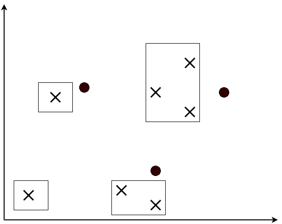
No matter how these points are labeled, we can always place a rectangle that separates differently labeled points.

However, when there are five points, shattering them with a rectangle is impossible. As a result, the VC dimension of axis-aligned rectangles is 4.

Using this, we can calculate the sample complexity with arbitrary $\epsilon$ and $\delta$ .

So, the class of 2D rectangles is PAC-learnable.

6.2. Class of Polynomial Classifiers In $\boldsymbol{\mathbb{R}}$

A classifier in a one-dimensional line can shatter at most 2 points, and a line in two-dimensional space can shatter at most 3 points. Similarly, the VC dimension of a polynomial classifier of degree $n$ is $n+1$ . As a result, each finite polynomial is PAC-learnable.

However, the class of all polynomial classifiers (i.e., their union) has a VC dimension of $\infty$ . Therefore, the union of polynomial classifiers is not PAC-learnable.

So, although any set of polynomials with the same finite degree is learnable, their union isn’t.

7. Conclusion

In this article, we gave an explanation of the PAC learning theory and discussed some of its main results.

In a nutshell, PAC learning is a theoretical framework investigating a relationship between the desired error rate and the number of samples for training a learnable classifier.

Full Archive

About Baeldung

Core Concepts

Operating Systems

Artificial Intelligence

Graph Theory

Latex