

Yes, we're now running our only Summer Sale. All Courses are 30% off until 20th July, 2026:
Learn through the super-clean Baeldung Pro experience:
>> Membership and Baeldung Pro.
No ads, dark-mode and 6 months free of IntelliJ Idea Ultimate to start with.
1. Introduction
Machine-learning algorithms come with implicit or explicit assumptions about the actual patterns in the data. Mathematically, this means that each algorithm can learn a specific family of models, and that family goes by the name of the hypothesis space.
In this tutorial, we’ll talk about hypothesis spaces and how to choose the right one for the data at hand.
2. Hypothesis Spaces
Let’s say that we have a binary classification task and that the data are two-dimensional. Our goal is to find a model that classifies objects as positive or negative. Applying Logistic Regression, we can get the models of the form:
(1) 
which estimate the probability that the object at hand is positive.
Each such model is called a hypothesis, while the set of all the hypotheses an algorithm can learn is known as its hypothesis space. In our case, a hypothesis could be  , while
  would be the hypothesis space.
2.1. Hypotheses and Assumptions
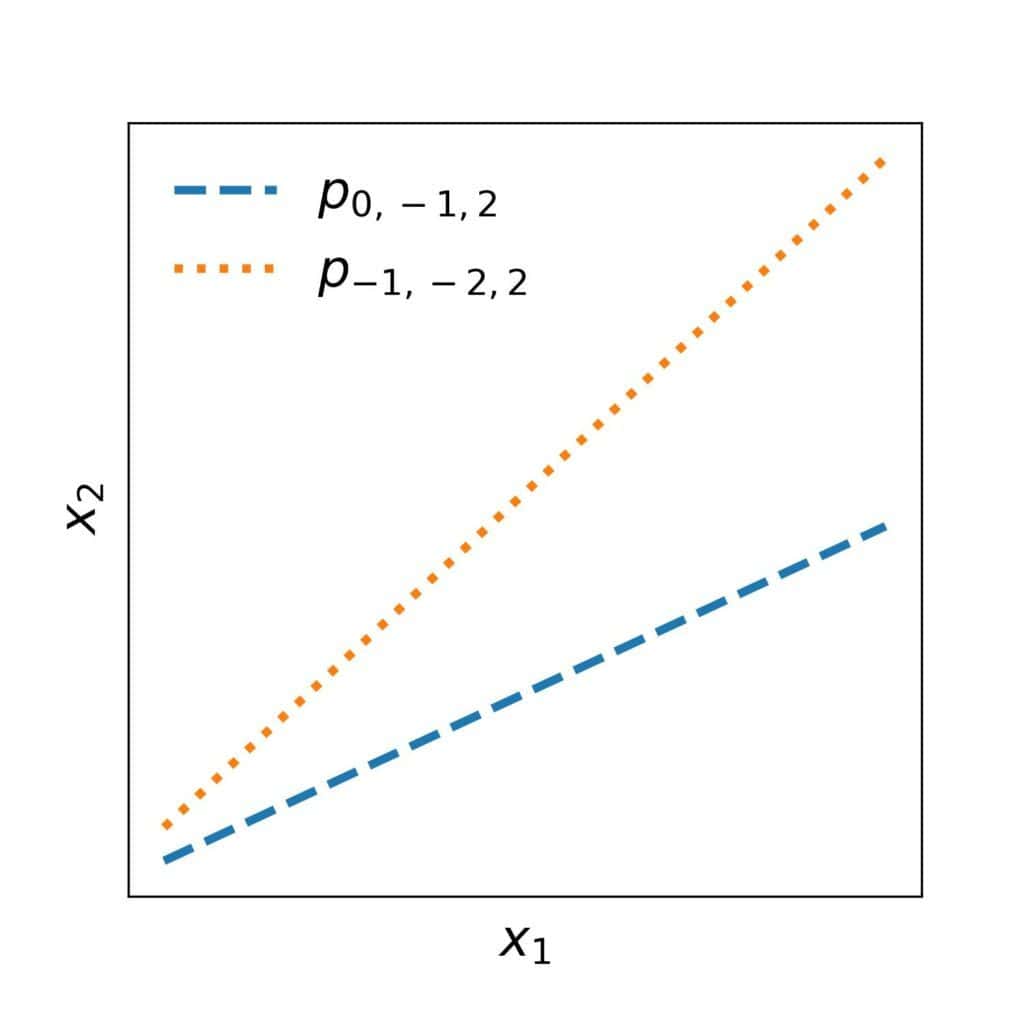
The underlying assumption of hypotheses (1) is that the boundary separating the positive from negative objects is a straight line. So, every hypothesis from this space corresponds to a straight line in a 2D plane. For instance:
2.2. Regression
Hypothesis spaces are present in regression problems as well. For example, Linear Regression assumes that the continuous outcome  is a linear combination of the features. So, if
  are the features, the hypotheses are of the form:
(2) 
3. Expressivity of a Hypothesis Space
We could informally say that one hypothesis space is more expressive than another if its hypotheses are more diverse and complex.
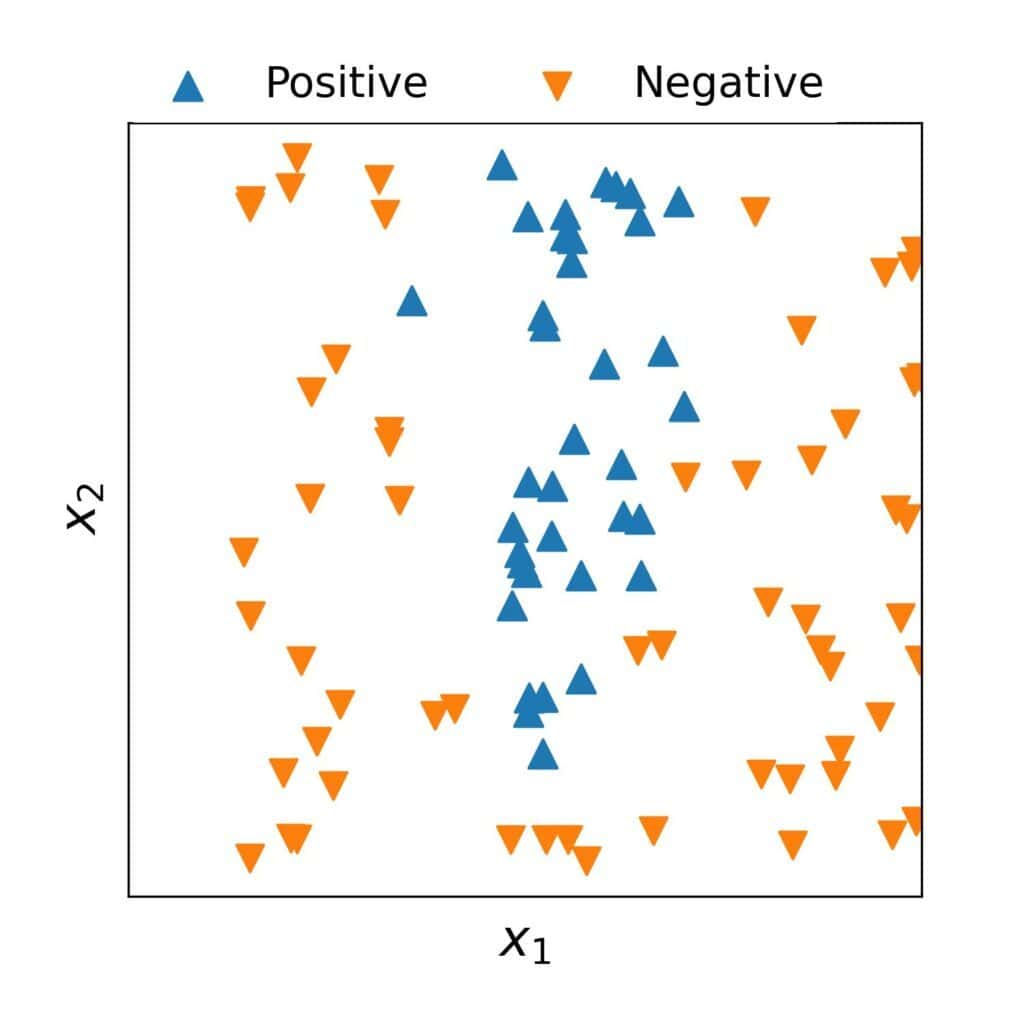
We may underfit the data if our algorithm’s hypothesis space isn’t expressive enough. For instance, linear hypotheses aren’t particularly good options if the actual data are extremely non-linear:
So, training an algorithm that has a very expressive space increases the chance of completely capturing the patterns in the data. However, it also increases the risk of overfitting. For instance, a space containing the hypotheses of the form:
(3) 
would start modelling the noise, which we see from its decision boundary:
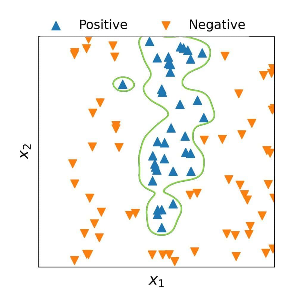
Such models would generalize poorly to unseen data.
3.1. Expressivity vs. Interpretability
Additionally, even if a complex hypothesis has a good generalization capability, it may be unusable in practice because it’s too complicated to understand or compute. What’s more, intricated hypotheses offer limited insight into the real-world process that generated the data. For example, a quadratic model:
(4) 
is easy to interpret: increases quadratically with  . However, what if we have a very complex model such as:
(5) 
It isn’t immediately apparent how depends on in that model.
4. How to Choose the Hypothesis Space?
We need to find the right balance between expressivity and simplicity. Unfortunately, that’s easier said than done. Most of the time, we need to rely on our intuition about the data.
So, we should start by exploring the dataset, using visualizations as much as possible. For instance, we can conclude that a straight line isn’t likely to be an adequate boundary for the above classification data. However, a high-order curve would probably be too complex even though it might split the dataset into two classes without an error.
A second-degree curve might be the compromise we seek, but we aren’t sure. So, we start with the space of quadratic hypotheses:
(6) 
We get a model whose decision boundary appears to be a good fit even though it misclassifies some objects:
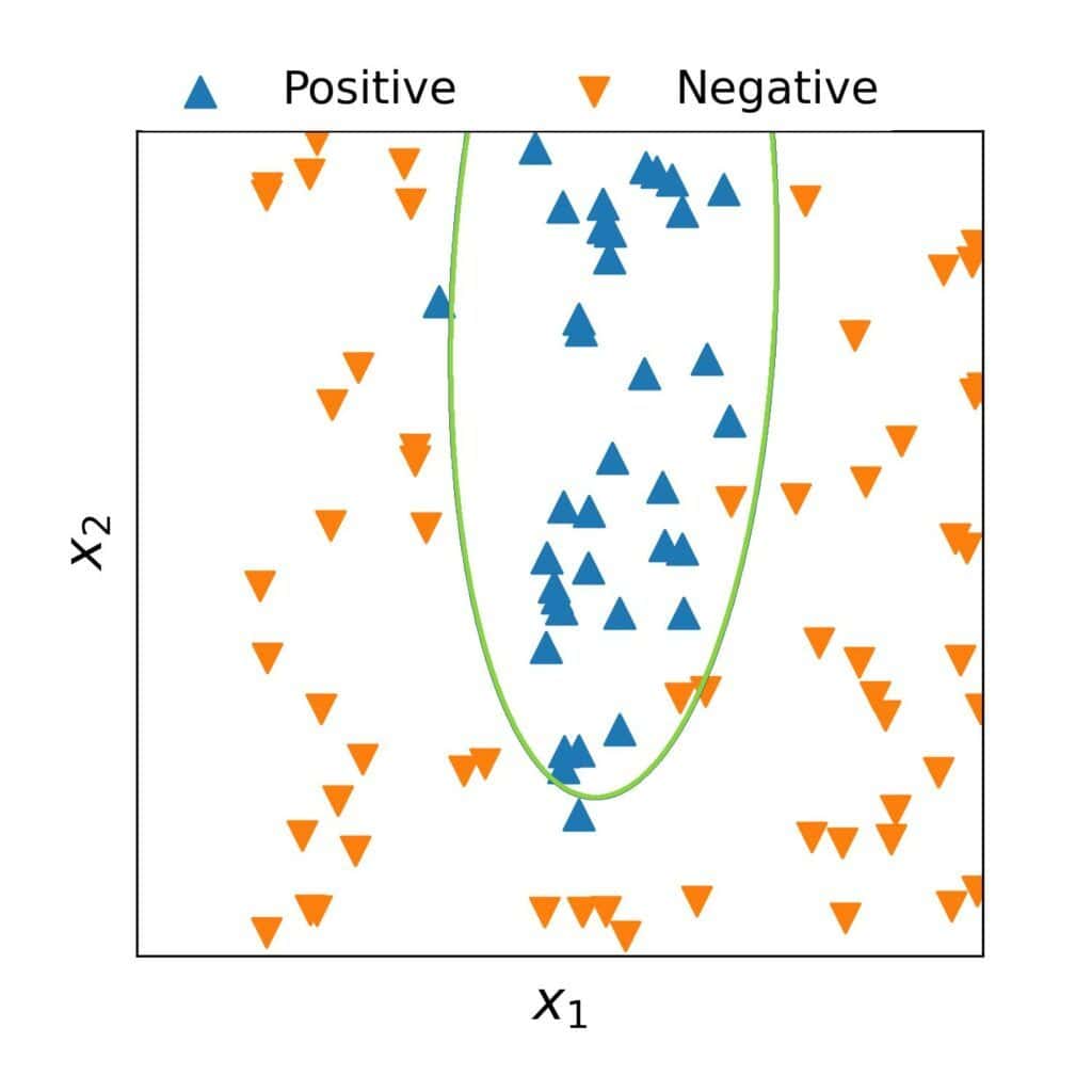
Since we’re satisfied with the model, we can stop here. If that hadn’t been the case, we could have tried a space of cubic models. The idea would be to iteratively try incrementally complex families until finding a model that both performs well and is easy to understand.
4. Conclusion
In this article, we talked about hypotheses spaces in machine learning. An algorithm’s hypothesis space contains all the models it can learn from any dataset.
The algorithms with too expressive spaces can generalize poorly to unseen data and be too complex to understand, whereas those with overly simple hypotheses may underfit the data. So, when applying machine-learning algorithms in practice, we need to find the right balance between expressivity and simplicity.