Rank of a Node in a Binary Search Tree | Baeldung on Computer Science

1. Introduction

In this tutorial, we’ll present three ways to determine the rank of a node in a binary search tree (BST).

2. A Node’s Rank in a Tree

The rank of a node value $\boldsymbol{x}$ in a tree is the number of the nodes whose values are $\boldsymbol{\leq x}$ . The nodes can be of any data type as long as it comes with an ordering relation $\leq$ . For example, the rank of $27$ in the following tree is $7$ :

So, we have a value $\boldsymbol{x}$ and the root of a tree, and the goal is to find the $\boldsymbol{x}$ ‘s rank in it.

We don’t assume that $x$ is present in the tree. If it is, it may repeat. The approaches we’ll present cover all the cases.

3. The Brute-Force Method to Determine Rank

The most obvious approach is to recursively calculate and add up the numbers of nodes with values $\leq x$ in the left and right sub-trees. If the root is $\leq x$ , we increment the sum by $1$ . If not, the sum is the rank of $x$ in the whole tree:

$rank(x, root) = \begin{cases} 0,& root \text{ is the root of an empty tree}\\ 1 + rank(x, root.left) + rank(x, root.right),& root \text{ isn't empty and } x \leq root.value\\ rank(x, root.left) + rank(x, root.right), & root \text{ isn't empty and } x > root.value \end{cases}$

3.1. Pseudocode

Here’s the pseudocode:

3.2. Example

Let’s see how this brute-force method calculates the rank of $27$ in the following tree:

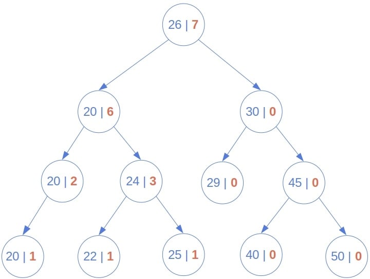
It goes all the way down to the leaves and recursively propagates the ranks of $27$ in the sub-trees until it gets to the root.

3.3. Complexity

This approach isn’t efficient. We always traverse the whole tree, so the time complexity is $\Theta(n)$ , where $n$ is the number of nodes. The reason is that we don’t use the fact that the tree is ordered.

4. Order-Based Calculation of Rank

There’s no need to calculate $rank\_right$ if $node.value > x$ because all the nodes in the right sub-tree are also greater than $x$ . So, we differentiate between two cases:

If $node.value \leq x$ , we should make recursive calls on both left and right sub-trees.
If $node.value > x$ , we can disregard the right sub-tree.

The pseudocode is as follows:

4.1. Example

This is how the order-based method determines the rank of $27$ :

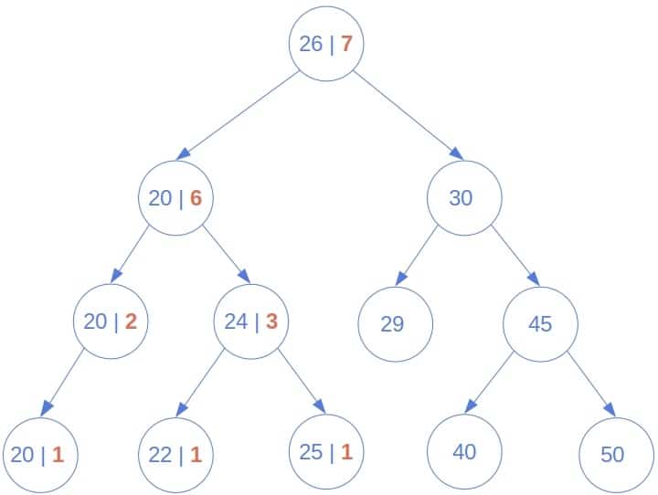
As we see, only the nodes less than or equal to $27$ were visited.

4.2. Complexity

The worst-case scenario happens when $x$ is greater than all the nodes in the tree. The algorithm will end up traversing the whole tree, so the worst-case time complexity is $\boldsymbol{O(n)}$ , the same as for the brute-force approach.

Still, the method will mostly run faster than brute force because it visits exactly $rank(x) \leq n$ nodes for any $x$ , whereas the brute-force solution visits $n$ nodes no matter the rank of $x$ .

We can, however, speed it up even more if we’re ready to do a little bookkeeping.

5. Order-Statistic Trees for Rank Calculation

If we augment each node with the information on its size, we can skip traversing the left sub-tree. Instead, we read the value of the size attribute and recurse on the right sub-tree only:

The trees whose nodes store the size can efficiently answer the queries about the rank of a value and find the node that has the given rank. Such trees are called order-statistic trees.

5.1. Example

Let’s see which nodes this algorithm will visit to determine the rank of $27$ :

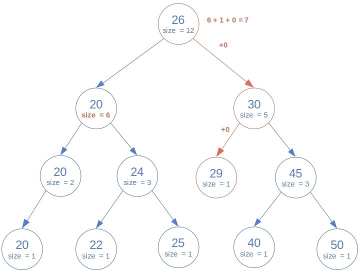
Since the root is $\leq 27$ , we read the size of its left sub-tree ( $6$ ), count the root as $\leq 27$ by adding $1$ to $6$ , and then recurse on the right sub-tree. The root of the right sub-tree ( $30$ ) is $>27$ so that we can disregard it along with its right descendants. Therefore, we make a recursive call for its left child. It’s also $>27$ , so we go to the left again. However, there’s no left child, so we return $0$ and propagate it to the root of the whole tree. That way, we calculate the rank as $6+1+0=7$ , which is the correct result.

5.2. Complexity

This method traverses a single path in the tree to find the input value’s rank. Any path’s length is bounded by $h$ , the tree’s height, i.e., the length of the longest path between the root and a leaf node. So, the time complexity is $\boldsymbol{O(h)}$ . Depending on the tree’s structure, $h$ is usually considerably lower than $n$ . But, the downside is that whenever we add or delete a node, we have to update the size attributes of all the node’s ancestors to the root.

If the tree is balanced, it will hold that $\boldsymbol{h=\Theta(\log n)}$ , so the whole algorithm will be of logarithmic complexity in the worst case. However, to keep the tree balanced, we need to rebalance it after every update.

If the tree is unbalanced, the worst case is the degenerate tree consisting of a single branch with $x$ larger than all the nodes. In that case, the algorithm will visit all $n$ nodes and have the worst-case complexity of $O(n)$ just like the other two approaches.

5.3. Tail-Recursive Rank Calculation

Unlike the previous two methods, this one can be made tail-recursive since there’s nothing with the return value of a recursive call other than passing it up the call stack. To transform the function to the tail-recursive form, we accumulate the partial results and make sure that the return statement is the last one executed in the function’s body:

Tail-recursive functions can be tail-call optimized, which means that a single frame on the call stack can be reused for each call. Without tail-call optimization, we risk the stack overflow error if the path being visited is too deep.

Further, there’s a straightforward way to turn tail-recursive functions into iterative ones.

6. Discussion

Which algorithm should we use? The answer is: it depends.

The brute-force approach is the least efficient of all the three but is sometimes the only way to go. If the tree is ordered by relation $\leq_a$ , and we want to find the rank for another relation $\leq_b$ , our only option is brute force. We have to traverse the whole tree because $x \leq_a node.value$ tells us nothing about $x \leq_b node.value$ (in general).

If we want to determine the rank for the same relation that orders the tree, the second and the third approaches will work better than brute force. If we can’t augment nodes with the size attribute, we should use the second algorithm. If we can, the third method should be our choice.

Whether or not we use the balanced trees depends on multiple factors. The first and the second algorithms don’t require balanced trees, but other operations we might perform on the tree may benefit if we keep it balanced. The third approach benefits the most from balancing the trees. But, due to rebalancing, it may not pay off. That’s the case if the rank queries are rare and insertions, deletions, and updates happen frequently.

7. Conclusion

In this article, we presented three ways to determine a node’s rank in a binary search tree. One is $O(\log n)$ if the input tree is balanced. Otherwise, all the three are $O(n)$ in the worst case, although the two non-brute-force approaches are typically faster than the brute-force method in practice.

Full Archive

About Baeldung

Core Concepts

Operating Systems

Artificial Intelligence

Graph Theory

Latex