Self-Balancing Binary Search Trees

1. Introduction

In this article, we’ll introduce the self-balancing binary search tree – a data structure that avoids some of the pitfalls of the standard binary search tree by constraining its own height. We’ll then have a go at implementing one popular variation – the left-leaning red-black binary search tree.

2. Binary Search Trees

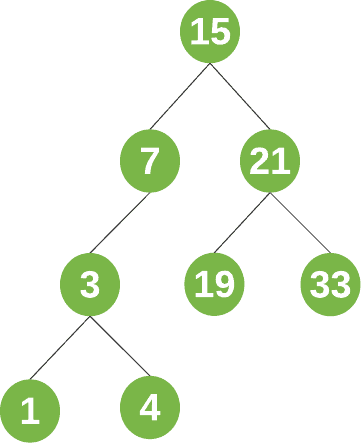
A binary search tree (BST) is a type of binary tree where the value at each node is greater than or equal to all node values in its left subtree, and less than or equal to all node values in its right subtree.

For example, a binary search might look like this:

There are a few key terms related to binary search tree:

• A leaf is a node with no children.
• The depth of a node refers to the number of nodes on the path from the root down to (and including) that particular node.
• The maximum depth of a binary tree refers to the depth of its deepest leaf. We can also refer to this measure as the tree height.
• A tree is balanced if, for every node in the tree, the height of its right and left subtrees differs by at most 1.

For a quick refresher on binary search trees, check out this article.

3. BST Operations

Typically, a binary search tree will support insertion, deletion, and search operations. The cost of each operation depends upon the height of the tree – in the worst case, an operation will need to traverse all the nodes on the path from the root to the deepest leaf.

A problem starts to emerge here if our tree is heavily skewed. For example, let’s consider this tree:

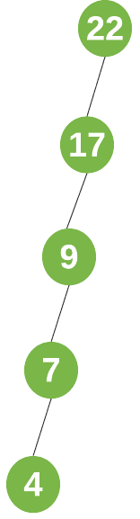
Whilst this is still a valid binary search tree, it clearly isn’t very useful. If we want to find, insert, or delete a node, we might end up traversing every node in the tree!

The worst-case cost of each operation on this tree is therefore $\bf{O(n)}$, for n number of nodes in the tree.

What we want instead, is a tree that is balanced.

A balanced tree is one where, for every node, the height of its right and left subtrees differs by at most 1. The height of a balanced tree is therefore bounded by $\bf{O(log_2n)$, meaning each operation will cost $\bf{O(log_2n)$ time in the worst case. This is a significant improvement from $O(n)$!

4. Self-Balancing BSTs

One way we can ensure our tree is always balanced is by implementing a self-balancing binary search tree. Such trees always keep their height to a minimum, ensuring that their operations will always maintain a worst-case cost of $\bf{O(log_2n)$.

There are a number of types of self-balancing BSTs. Each type varies slightly, but the main idea is that we check to see whether the tree has remained balanced after any state change – that is, any insertion or deletion on the tree. If it isn’t, we automatically perform some transformations on the tree to return it to a balanced/legal state.

Let’s take a look at one particular type of self-balancing Binary Search Tree: the Left-Leaning Red-Black BST.

5. Left-Leaning Red-Black BST

The left-leaning red-black tree keeps its height to a minimum by enforcing a couple of properties:

1. Each edge in the tree is colored red or black
2. Nodes may only touch one red edge
3. The number of black edges from the root to each empty leaf node is equal

When these properties hold, that is, when the tree is in a “legal” state, the height of the tree can be at most $2\log_2 n$. But how can we maintain a legal state?

5.1. Maintaining Balance

We do this by simply checking that each property holds after any insertion or deletion operation. If the tree has become unbalanced, we perform some transformations to return the tree to a legal state.

More specifically, there are three types of transformations we perform on our tree nodes:

1. Left rotation
2. Right Rotation
3. Color flip

Let’s take a closer look at these transformations and implement each one.

5.2. Left Rotation

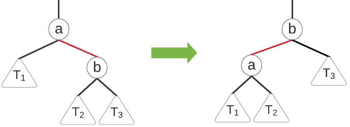
For this transformation, we perform a single left rotation to switch the direction of a red link. We can visualize the process:

And we might write the pseudocode as:

algorithm LEFT_ROTATE(node):
    // INPUT
    //    node = the node to rotate around
    // OUTPUT
    //    the tree after performing a left rotation on the given node

    x <- node.right
    node.right <- x.left
    x.left <- node
    
    x.color <- node.color
    node.color <- RED
    
    return x

5.3. Right Rotation

This transformation is just the reverse of our left rotation:

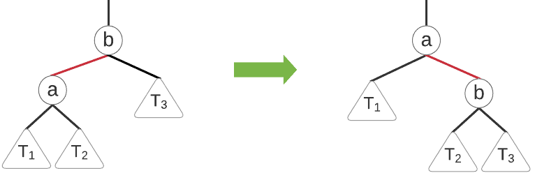
Our pseudocode for this transformation is therefore:

algorithm RIGHT_ROTATE(node):
    // INPUT
    //    node = the node to rotate around
    // OUTPUT
    //    the tree after performing a right rotation on the given node

    x <- node.left
    node.left <- x.right
    x.right <- node
    
    x.color <- node.color
    node.color <- RED
    
    return x

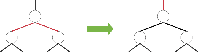
5.4. Color Flip

The color flip handles the illegal state where two adjacent red links are touching a node. In this case, we effectively swap the color of our two links with the single link above. Now, this local state is legal:

We can implement this function as follows:

algorithm COLOR_FLIP(node):
    // INPUT
    //    node = the node to perform a color flip on
    // OUTPUT
    //    the node after swapping the colors of its children and itself

    node.color <- RED
    node.left.color <- BLACK
    node.right.color <- BLACK

5.5. Is Red Function

It turns out that implementing some sequence of these three rotations can always return the tree to a legal state. Pretty neat!

There is one more helper function we need for our red-black tree: the IS-RED function. This simply tells us whether or not a node is red:

algorithm IS_RED(node):
    // INPUT
    //    node = the node to check color of
    // OUTPUT
    //    true if the node is red, false otherwise

    if node.color = RED or node = null
        return true
    else:
        return false

5.6. Insertion into the Red-Black Tree

Using the helper functions we defined above, we can now implement our red-black tree.

We’ll look at insertion first. As we mentioned previously, inserting a node into a red-black tree mostly mimics the standard BST insertion. We just have one extra step: after the insertion, we check to make sure our tree is still “legal”, and if not, we need to employ a sequence of transformations to return it to a “legal” state.

So, we have our transformation functions. But how do we decide what sequence of functions we need to implement, to re-balance the tree? Surely there are many cases to consider.

Well, in fact, it only takes a few lines of code to cover all of these cases. Let’s take a look:

algorithm INSERT(value, node):
    // INPUT
    //    value = the value to insert
    //    node = the current node in the tree
    // OUTPUT
    //    the node after insertion, ensuring the red-black tree properties

    if node = null:
        return new node(value, RED)
    else:
        if value <= node.value:
            node.left <- INSERT(node.left, value)
        else if value > node.value:
            node.right <- INSERT(node.right, value)

        if IS_RED(node.right) and not IS_RED(node.left):
            node <- LEFT_ROTATE(node)
        if IS_RED(node.left) and not IS_RED(node.left.left):
            node <- RIGHT_ROTATE(node)
        if IS_RED(node.left) and not IS_RED(node.right):
            COLOR_FLIP(node)

        return node

5.7. Operation Cost

When these properties hold, the height of the tree can be no greater than 2log₂n. Also, each rotation only costs us constant time.

Therefore, the worst-case cost of insert, delete, and search operations in the red-black tree will be bound by $\bf{O(2log_2n) = O(log_2n)}$. The best-case and average-case complexities are also bound by $O(\log_2 n)$.

6. Conclusion

In this article, we saw how binary search trees can dramatically improve their worst case costs by implementing some self-balancing.

We saw how a few lines of code can take a standard binary search tree and make it self-balancing red-black BST.