Neural Networks: Pooling Layers | Baeldung on Computer Science

1. Introduction

In this tutorial, we’ll walk through pooling, a machine-learning technique widely used that reduces the size of the input and, thus the complexity of deep learning models while preserving important features and relationships in the input data. In particular, we’ll introduce pooling, explain its usage, highlight its importance, and give brief examples of how it works.

2. What Are Pooling Layers?

In machine learning and neural networks, the dimensions of the input data and the parameters of the neural network play a crucial role. So this number can be controlled by the stacking of one or more pooling layers.

Depending on the type of the pooling layer, an operation is performed on each channel of the input data independently to summarize its values into a single one and thus keep the most important features. These values are driven as input to the next layer of the model and so on. The pooling process may be repeated several times, and each iteration reduces the spatial dimensions. The value aggregation can be performed by using different techniques.

3. Types of Pooling Layers

There are many pooling operations and different extensions that have been developed to address specific challenges in different applications.

3.1. Max Pooling

Max pooling is a convolution technique that chooses the maximum value from the patch of the input data and summarizes these values into a feature map:

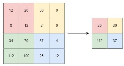
max pooling with a 2x2 window and stride 2

This method maintains the most significant features of the input by reducing its dimensions. The mathematical formula of max pooling is:

$\begin{equation*} \text{MaxPooling}(X)_{i,j,k} = \max_{m,n} X_{i \cdot s_x + m, j \cdot s_y + n, k} \end{equation*}$

where $X$ is the input, $(i,j)$ are the indices of the output, $k$ is the channel index, $s_x$ and $s_y$ are the stride values in the horizontal and vertical directions, respectively, and the pooling window is defined by the filter size $f_x$ and $f_y$ centered at the output index $(i,j)$ .

3.2. Average Pooling

Average pooling calculates the average value from a patch of input data and summarizes these values into a feature map:

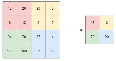
average pooling with a 2x2 window and stride 2

This method is preferable in cases in which smoothing the input data is necessary as it helps to identify the presence of outliers. The mathematical formula of average pooling is:

$\begin{equation*} \text{AvgPooling}(X)_{i,j,k} = \frac{1}{f_x \cdot f_y}\sum_{m,n} X_{i \cdot s_x + m, j \cdot s_y + n, k} \end{equation*}$

3.3. Global Pooling

Global pooling summarizes the values of all neurons for each patch of the input data into a feature map, regardless of their spatial location. This technique is also used to reduce the dimensionality of the input and can be performed either by using the maximum or average pooling operation. The mathematical formula of global pooling is:

$\begin{equation*} \text{GlobalPooling}(X)_{k} = f(X{:,:,k}) \end{equation*}$

where $X$ is the input, $k$ is the channel index, and $f$ is a function that aggregates the values in the feature map into a single value, such as average or max pooling, that was introduced before.

3.4. Stochastic Pooling

Stochastic pooling is a deterministic pooling operation that introduces randomness into the max pooling process. This technique helps in improving the robustness of the model to small variations in the input data. The mathematical formula of stochastic pooling is:

$\begin{equation*} \text{StochasticPooling}(X)_{i,j,k} = \begin{cases} X_{i,j,k} & \text{with probability } p_{i,j} \\0 & \text{with probability } 1 - p_{i,j} \end{cases} \end{equation*}$

where $X$ is the input, $(i,j)$ are the indices of the output tensor, $k$ is the channel index, and $p_{i,j}$ is the probability of retaining the value at position $(i,j)$ in the input feature map. The probabilities are generated randomly for each pooling window and are typically proportional to the values in the window.

4. Advantages and Disadvantages

In machine learning, pooling layers offer several advantages and disadvantages as well.

First of all, pooling layers help in keeping the most important characteristics of the input data. Furthermore, the addition of pooling layers in the neural network offers translation invariance, which means that the model can generate the same outputs regardless of small changes in the input. Moreover, these techniques help in reducing the impact of outliers.

On the other hand, the pooling processes may lead to information loss, increased training complexity, and limited model interpretability.

The main benefits and limitations are summarized in the table below:

5. Usages of Pooling Layers in Machine Learning

Pooling layers play a critical role in the size and complexity of the model and are widely used in several machine-learning tasks. They are usually employed after the convolutional layers in the convolutional neural network’s structure and are mainly used for downsampling the output.

These techniques are commonly used in convolutional neural networks and deep learning models of computer vision, speech recognition, and natural language processing.

6. Conclusion

In conclusion, pooling layers play a critical role in reducing the size and complexity of deep learning models while preserving important features and relationships in the input data.

In this article, we walked through pooling layers, a powerful and widely used technique in machine learning that offers many advantages for a wide range of applications. In particular, we introduced pooling layers, mentioned the most common pooling techniques, and summarized their main benefits and limitations.

Full Archive

About Baeldung

Core Concepts

Operating Systems

Artificial Intelligence

Graph Theory

Latex