

Yes, we're now running our only Summer Sale. All Courses are 30% off until 20th July, 2026:
Learn through the super-clean Baeldung Pro experience:
>> Membership and Baeldung Pro.
No ads, dark-mode and 6 months free of IntelliJ Idea Ultimate to start with.
1. Introduction
In this tutorial, we’ll talk about the channels of a Convolutional Neural Network (CNN) and the different techniques that are used to modify the input images.
A CNN is a class of artificial neural networks (ANN), mainly applied in machine learning areas like pattern recognition and image analysis and processing.
2. Convolution
First of all, a digital image is a bi-dimensional representation of pixels in rectangular coordinates. Therefore, every image consists of pixels, and each pixel is a combination of primary colors.
A convolution is an operation with two images (matrices). Therefore, a matrix is treated by another one, referred to as the kernel. Depending on the desired image effect, the kernel that is applied to the input image varies significantly.
The definition of 2D convolution and the mathematical formula on how to convolve is:
(1) ![\begin{equation*} \begin{aligned} y[m, n] = x[m, n] * h[m, n] = \sum_{j = - \infty}^{\infty} \sum_{i = - \infty}^{\infty} x[i, j] \cdot h[m-i, n-j] \end{aligned} \end{equation*}](/wp-content/ql-cache/quicklatex.com-4331a2dca1e6f440e5135b356beced1f_l3.svg "Rendered by QuickLaTeX.com")
where  and
and  denote the representation of pixels in rectangular coordinates, the filter applied, the output of the convolution, and the dimensions of the image and filter respectively.
2.1. Different Types of Kernels
Depending on the desired effect, a kernel may cause different effects on an image.
- Blurring: Produces a kernel in which the centered pixels contribute more information than those near the edges.
- Sharpening: Produces a kernel that sharpens the image and enhances its acutance.
- Embossing: Produces a kernel in which every pixel is replaced either by a highlight or a shadow.
- Edge Detection: Produces a kernel that identifies the edges within an image to detect the boundaries of objects in it.
Besides the above, many different kernels may cause various modifications to an input image.
2.2. Example of Convolution
Let’s assume that we have an image that can be represented as a matrix in which every pixel contains a value.
![\[\begin{bmatrix} 1 & 2 & 3 \\ 4 & 5 & 6 \\ 7 & 8 & 9 \end{bmatrix}\]](/wp-content/ql-cache/quicklatex.com-04e0944bdc8588a6a1d2e2e49924dc06_l3.svg "Rendered by QuickLaTeX.com")
Suppose that we choose to modify this image with a kernel to achieve certain effects on it.
![\[\begin{bmatrix} -1 & -2 & -1 \\ 0 & 0 & 0 \\ 1 & 2 & 1 \end{bmatrix}\]](/wp-content/ql-cache/quicklatex.com-173ee6cc8423d5a06a279cf97e5f202c_l3.svg "Rendered by QuickLaTeX.com")
The computation of the first element of the output matrix, according to the formula above:
(2) ![\begin{equation*} \begin{aligned} y[0, 0] = \sum_{j} \sum_{i} x[i, j] \cdot h[0 - i, 0 - j] = x[-1, -1] \cdot h[1, 1] + x[0, -1] \cdot h[0, 1] \\+ x[1, -1] \cdot h[-1, 1] +x[-1, 0] \cdot h[1, 0] + x[0, 0] \cdot h[0, 0] + x[1, 0] \cdot h[-1, 0] + x[-1, 1] \cdot h[1, -1] \\+ x[0, 1] \cdot h[0, -1] + x[1, 1] \cdot h[-1, -1] = 0 \cdot 1 + 0 \cdot 2 + 0 \cdot 1 + 0 \cdot 0 + 1 \cdot 0 + 2 \cdot 0 + 0 \cdot (-1) \\+ 4 \cdot (-2) + 5 \cdot (-1) = -13 \end{aligned} \end{equation*}](/wp-content/ql-cache/quicklatex.com-cb8556ac729115b4e259ed85af941af3_l3.svg "Rendered by QuickLaTeX.com")
We compute the convolution operations similarly.
![\[\begin{bmatrix} 1 & 2 & 3 \\ 4 & 5 & 6 \\ 7 & 8 & 9 \end{bmatrix} * \begin{bmatrix} -1 & -2 & -1 \\ 0 & 0 & 0 \\ 1 & 2 & 1 \end{bmatrix} = \begin{bmatrix} -13 & -20 & -17 \\ -18 & -24 & -18 \\ 13 & 20 & 17 \end{bmatrix}\]](/wp-content/ql-cache/quicklatex.com-4d3928c65186c7bd1da3f7e34f8e63d4_l3.svg "Rendered by QuickLaTeX.com")
As we can see in the image below the filter (deep blue) is applied to the input image (blue) and results in the convolution’s output (green image):
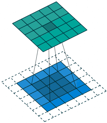
Note that, in case we apply more than one convolutional kernel, many channels are produced, one from each convolutional kernel.
3. Channel Input
In machine learning, neural networks perform image processing on multi-channeled images. Each channel represents a color, and each pixel consists of three channels. In a color image, there are three channels: red, green, and blue. An RGB image can be described as a  matrix, where
  ,
,  , and
, and  denote the width, height, and the number of channels respectively. Thus, when an RGB image is processed, a three-dimensional tensor is applied to it.
Unlike RGB images, grayscale images are singled channeled and can be described as a  matrix, in which every pixel represents information about the intensity of light.
4. Convolutional Layers
Convolutional layers typically involve more than one channel, where each channel of a layer is associated with the channels of the next layer and vice versa. The basic structure of a CNN model is composed of convolutional layers, pooling layers:
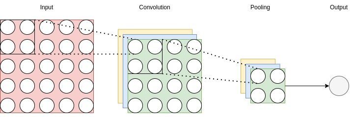
A convolution layer receives a input image and produces an output that consists of an activation map, as we can see in the diagram above, where and are the width and height, respectively. The filter for such a convolution is a tensor of dimensions  , where
  is the filter size which normally is 3, 5, 7, or 11, and is the number of channels. The depth of the convolution matrices in the convolution network is the total number of channels and must always have the same number of channels as the input. Therefore, a greater channel depth would lead to the reduction of spatial resolution.
5. Feature Techniques
It’s helpful to mention certain techniques that are widely used in convolution layers: Pooling, Padding, and Strides.
5.1. Pooling
Most CNN architectures include an operation that is called Pooling. Pooling is a widely used technique that mainly focuses on reducing the dimensions of the feature maps. Therefore, the addition of pooling filters accelerates the performance of the neural network and leads to faster training because it lessens the number of parameters that the CNN has to learn and leads to smaller outputs.
In addition, pooling filters help to learn the most crucial features and remove outliers and invariances.
There have been proposed different for pooling. The most widespread and widely used are max and average pooling.
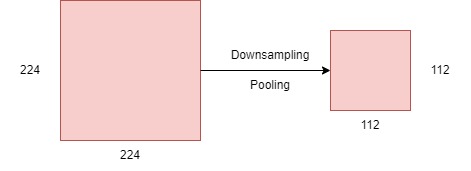
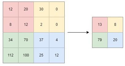
Pooling involves downsampling an input image and, reducing its dimensionality:
5.2. Max Pooling
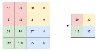
Maximum pooling is a pooling technique that computes the largest value in each windowed patch. The filter simply picks the maximum pixel value in the receptive field of the feature map. For example, if we have 4 pixels in the field (red) with values 12, 20, 8, and 12, we select 20.
5.3. Average Pooling
Average pooling is a pooling technique that computes the average value of the pixel values in the windowed patch. For example, if we have 4 pixels in the field (red) with values 12, 20, 8, and 12, an average pooling filter would lead to 13.
5.4. Padding
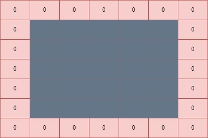
Apart from pooling, most CNN architectures include an operation that is called Padding. Padding is also a widely used method that settles the number of pixels that are appended to an input image. It is a useful technique when a CNN needs to process an image in an extended format. Increasing the number of pixels in an image leads to more accurate results in the learning phase of the CNN, as the pixels of the border, which usually contribute less, tend to get closer to the middle.
In a CNN, if zero padding is applied, then the borders of the image will be filled with pixels of value zero. A  image with
  layer of zero padding is:
5.5. Stride
Stride is a parameter of the neural network’s filter that is used for data compression. It denotes the number of steps of the shifting of a convolutional filter over an input image or video. In other words, stride manages how far the filter moves across an image in every step in one direction by adjusting the number of units that have to be made in order for the filter to move through the input image.
In a CNN, if a neural network’s stride is set to two, the filter will slide by two pixels, or units, at a time. Therefore, certain locations of the kernel and input image are skipped. Stride can lead to smaller activation maps, which improves the CNN’s performance and execution time. However, on certain occasions, it may lead to information loss.
 and
and  would result to a
  and
and  feature map respectively:
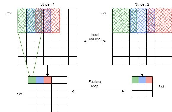
As we can see slides the filter faster through the image and produces fewer results on the feature map.
6. Conclusion
In this article, we walked through Convolutional Neural Networks. In particular, we discussed in detail the channels of the Convolutional Neural Network and talked over some techniques that are used on the image inputs.