

Yes, we're now running our only Summer Sale. All Courses are 30% off until 20th July, 2026:
Trade-offs Between Accuracy and the Number of Support Vectors in SVMs
Last updated: February 13, 2025
Learn through the super-clean Baeldung Pro experience:
>> Membership and Baeldung Pro.
No ads, dark-mode and 6 months free of IntelliJ Idea Ultimate to start with.
1. Introduction
In this tutorial, we’ll study the relationship between the number of support vectors and the performance of a support vector classifier.
We’ll begin with some notes on support vector machines and their decision boundaries in classification problems.
Then, we’ll study the variation in the level of accuracy of a classifier, in relation to the value assumed by the regularization parameter and the number of support vectors. We’ll do so in a concrete case, related to a typical dataset for machine learning.
At the end of this tutorial, we’ll know the heuristic for determining the trade-offs between accuracy and the number of support vectors for a support vector classifier.
2. Support Vector Machines and Classification Problems
2.1. Support Vector Machines and Support Vectors
In our other tutorials on this website, we have previously studied support vector machines in their general theoretical foundations. We have also compared them with neural networks, to which SVMs are to some extent analogous. Finally, we have also studied the advantages and disadvantages of the two models in performing some specific machine learning tasks.
We can refer to those tutorials if we need a refresh. Here, we want to instead focus on optimizing support vector machines for classification tasks. The problem of optimizing a support vector machine corresponds to the problem of identifying its hyperparameters, such that the accuracy of the classification is maximized and the number of support vectors is minimized, ideally at the same time.
Because a support vector machine is configured according to two hyperparameters, the type of the kernel and the so-called regularization parameter, we need a technique that lets us compare the trade-offs between accuracy and the number of support vectors, as the kernel is changed and as the regularization parameter  varies. Our problem, therefore, consists in identifying a method for studying the four-dimensional system that we call the support vector machine:

In this model, we can think of our task as the challenge of selecting a kernel and a regularization parameter that, given a particular dataset, gives us the highest accuracy while keeping the number of support vectors contained.
2.2. What Functions Do Support Vectors Have?
We know that a support vector machine is guaranteed to find a decision boundary for the separation of data into classes. This, of course, for an appropriate choice of its kernel.
The reason why this happens is that SVMs learn to separate the observations that are the closest to one another in their feature space. The question then becomes: how can we obtain the highest possible accuracy on a dataset, while simultaneously minimizing the number of support vectors?
2.3. The Shape of the Decision Boundary
One way to look at this problem is to consider the support vectors that an SVM chooses as some sort of assumption that the model makes regarding the shape of the decision boundary. These assumptions are considered to be more binding, or more specific, than those corresponding to the general distribution of the data.
Let’s take an example to clarify this concept. It’s always beneficial, when considering a theoretical problem, to reason about the simplest or edge cases that that problem entails. We can begin with a dataset comprising two observations and two classes:

This problem is linearly separable. An SVM with a linear kernel would therefore learn the hyperplane that maximally separates these observations, which in this case is a line:

2.4. When the Number of Observations Increases
The SVM, in this example, uses 100% of the observations as support vectors. As it does so, it reaches maximum accuracy, whichever metric we want to use to assess it. The number of support vectors can however not be any lower than 2, and therefore this quantity does not appear problematic.
As the number of observation increases, however, we may decide that a line that separates strictly the two classes may no longer suit us:

This is because, if the number of observations is not trivial unless the problem preserves its linear separability, we’ll generally need to accept more sophisticated decision boundaries:

If we don’t, we’re going to lose inaccuracy. If we do, we’re going to rely on an increased number of support vectors. Either way, we’re obligated to conduct trade-offs between the two.
3. A Concrete Example
3.1. Preliminary Data Analysis
We can now study the concrete implementation of a SVM, for the purpose of modeling a common dataset for machine learning. As we do that, we’ll observe and note the way in which the number of support vectors chosen by the SVM affects both the accuracy and the shape of the decision boundary thereof.
The experiment that we discuss here is based upon the Iris dataset, which is a standard dataset for machine learning:
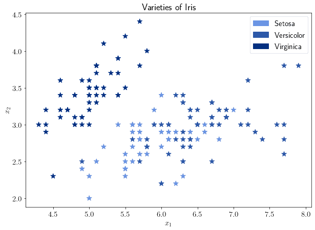
If we take two out of the four features associated with each observation, we can intuitively note how one of the classes is located in its own region of the feature space, while the other two aren’t. This strongly suggests that a linear kernel for the SVM may not be the most appropriate kernel unless we choose soft margins and a regularisation parameter that allows for a sufficient number of support vectors to be chosen.
The question then becomes: how do we choose the regularisation parameter that gives us the best trade-off, between the number of support vectors and the accuracy of the classifier for this particular dataset?
3.2. Linear Kernels
This type of question can be solved by studying the way in which the accuracy of the classifier and the number of support vectors change, as we modify slightly the regularization parameter. Let’s begin by considering the standard value of the regularization parameter; in this case,  :
:
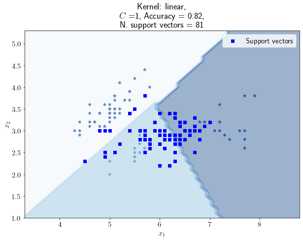
From here onward, as an accuracy metric, we’ll always be using the Jaccard score. If the regularization parameter is 1, the SVM uses 81 support vectors and has an accuracy of 0.82, in order to classify the flowers of the Iris dataset.
3.3. Let’s Change the Regularization Parameter
Now, if we decrease a little, we’d expect the number of support vectors to increase. This is because the regularization parameter is inversely proportional to the strength of the regularization process. And indeed, if we set to 0.1, we obtain this:
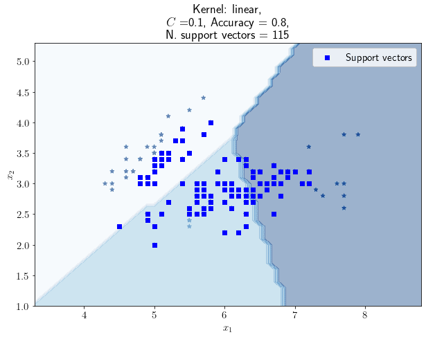
The number of support vectors has gone up to 115, but the accuracy score has decreased to 0.80. This is because, as mentioned earlier, two of the classes occupy overlapping regions of the feature space. As the number of support vectors increases, the decision boundary to the bottom-right of the picture is moved slightly to the left, and more observations are thus incorrectly classified.
If we invert the line of reasoning, we may also expect the number of support vectors to go down, as the parameter increases. For a value of equal to 10, for example, we obtain this graph:
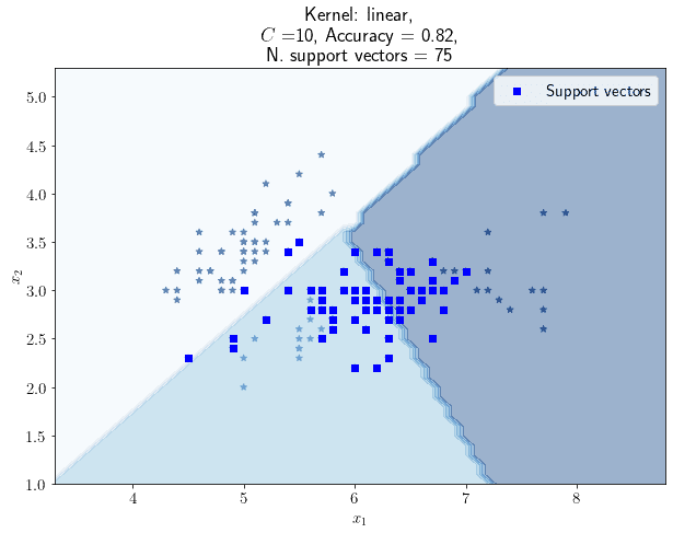
The number of support vectors, in this case, is 75 which is the lowest we recorded so far. The accuracy, however, is 0.82 which is not higher than the one we observed for . We might be interested to see if, by incrementally reducing the value of , we get to some higher values for the accuracy or some lower values for the number of support vectors, or both. As a general rule, we’d expect the accuracy to go up as the number of support vectors goes up, but this may not always be the case.
3.4. Accuracy and Number of Support Vectors
We can then replicate the procedure we followed above, by increasing and decreasing the value of . In doing so, we can study the relationship that exists between the value of , the number of support vectors that are identified, and the resulting accuracy score.
For this particular experiment, we tested all values of contained in the interval  and sampled with a resolution of 0.01. This is the resulting chart:
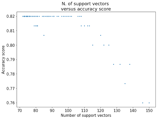
Notice how the accuracy score never jumps over a certain value, 0.82 in this case. This is because the problem is intrinsically non-linearly separable. We, therefore, need to live with the idea that some observations will always be incorrectly classified by an SVM with a linear kernel.
Notice also, however, that increasing the number of support vectors does not necessarily increase the performance of the classifier. In fact, it seems that the trade-off between the number of support vectors and the accuracy that we believed to be true does not necessarily apply to this particular case. If the number of support vectors is already above a certain threshold, around 110 in this case, then there are decidedly decreasing marginal returns that derive from the choice of an additional support vector.
3.5. Non-Linear Kernels
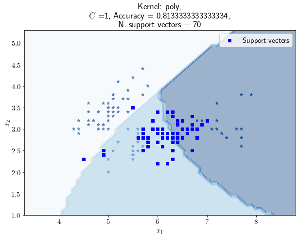
Because we believe that the lower accuracy observed for this problem, as the number of support vectors increase, is dependent upon the non-linear separability of the problem itself, it then makes sense to use SVMs with non-linear kernel and see what happens to their accuracy as we change . We’d expect, in general, an SVM with a non-linear kernel to perform better than a linear SVM. For this experiment, we chose an SVM with a polynomial kernel of degree 3. Here is its graph for :
As we did earlier, we can then shift the value of up and down and keep track of the corresponding accuracy score and the number of support vectors. For simplicity, we won’t report any other individual cases. Instead, here are the results of the training for all values of  , with a resolution of 0.01:
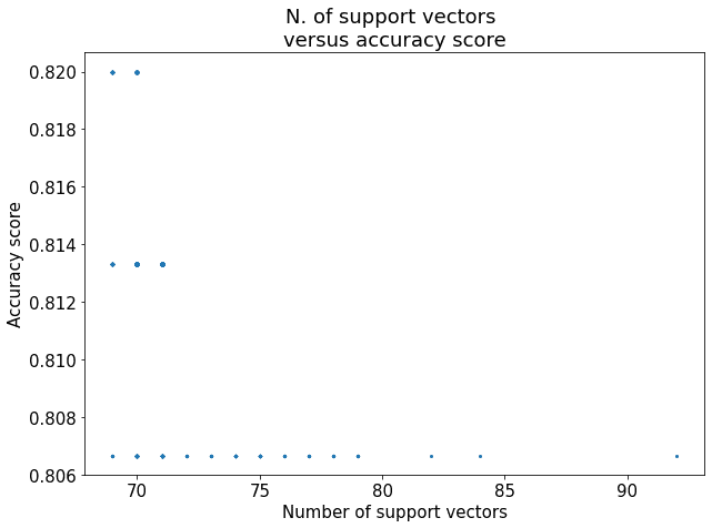
As we can see from this graph, the lowest value observed for the accuracy of a polynomial SVM is higher than the lowest value we obtained with a linear SVM. This suggests that, for this particular problem, the non-linear SVM performs slightly better, as we expected.
3.6. Accuracy with Minimal Number of Support Vectors
We can also notice, though, that increasing the number of support vectors for the polynomial SVM leads to decreased accuracy much sooner than was observed with a linear SVM. In particular, we can see how we have a marked drop in accuracy if the number of support vectors is higher than 70, which is much lower than the value of 110 that we observed in the previous case.
Because the highest accuracy score, 0.82, is observed only for a number of support vectors corresponding to 69 or 70, we can move to study the relationship between the regularisation parameter and the associated accuracy, when the number of support vectors is either 69 or 70:
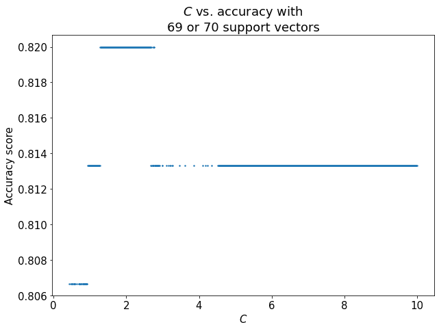
We can see that there is a sweet spot for  for which, notwithstanding the invariance in the number of support vectors, the accuracy is maximized. This is all the information we need, in order to decide what is the most optimal trade-off between the accuracy of the classifier and the number of support vectors.
3.7. So, Which Kernel and Which Regularization?
For the considerations we made here, it makes therefore sense to use a non-linear kernel for this particular problem. This is because, if we compare the distributions of accuracies versus the number of support vectors for a linear and a non-linear kernel, the non-linear kernel is generally more accurate and uses fewer support vectors:
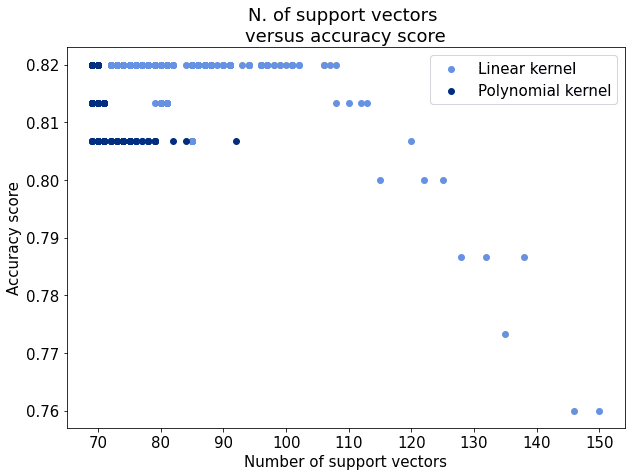
Upon choosing the type of kernel, we can also decide on the optimal value of the regularization parameter. In the previous section, we saw that, for the polynomial kernel, the accuracy was maximized and the number of support vectors was minimized, simultaneously, for a value of corresponding to approximately 2. That is to say, for this particular dataset the best approach would be to select a non-linear kernel with that particular regularization parameter.
3.8. What About Other Datasets?
The methodology that we have discussed here is not specific to this particular problem. It falls, instead, under the general category of machine learning heuristics. Knowing the collection of heuristics is important when we’re confronted with the problem of optimizing the hyperparameters of a machine learning model.
In this specific case, we solved this problem by manually conducting the operation of testing and assessing the possible values that the parameters of the model can assume. More generally, though, we may want to apply automated methods for searching the hyperparametric configuration of a model, such as by applying grid search.
Then, we assessed manually which combination of the accuracy score and size of the model satisfied our needs. We were lucky to find that it is possible to maximize accuracy and minimize the size for some particular configuration. This may however not always be the case, and therefore caution is advised.
4. Conclusions
In this article, we studied the relationship between the number of support vectors and the performances of a support vector classifier.
We initially discussed the role that support vectors have in determining the shape of the decision boundary. We’ve also introduced the idea that increases in accuracy and decreases in the number of support vectors can be traded for one another.
Finally, we’ve applied the previous considerations to the study of the performances of an SVM classifier on a famous dataset for machine learning.