Minimum Cut on a Graph Using a Maximum Flow Algorithm

1. Overview

In this tutorial, we’ll discuss how to find the minimum cut of a graph by calculating the graph’s maximum flow. We’ll describe the max-flow min-cut theorem and present an algorithm to find the maximum flow of a graph.

Finally, we’ll demonstrate the algorithm with an example and analyze the time complexity of the algorithm.

2. Minimum Cut in a Graph

In general, a cut is a set of edges whose removal divides a connected graph into two disjoint subsets. There are two variations of a cut: maximum cut and minimum cut. Before discussing the max-flow min-cut theorem, it’s important to understand what a minimum cut is.

Let’s assume a cut $CT(S, T)$ partition the vertex set $V$ into two sets $S,$ and $T$ . The net flow $f(S, T)$ of a cut $CT(S, T)$ can be defined as the sum of flow $f(u, v)$ , where $u, v$ are two nodes $\in V$ , and $u \in S, v \in T$ . Similarly the capacity $C(u, v)$ of a cut $CT(S, T)$ is the sum of the individual capacities, where $u, v$ are two nodes $\in V$ , and $u \in S, v \in T$ .

The minimum cut of a weighted graph is defined as the minimum sum of weights of edges that, when removed from the graph, divide the graph into two sets.

Let’s see an example:

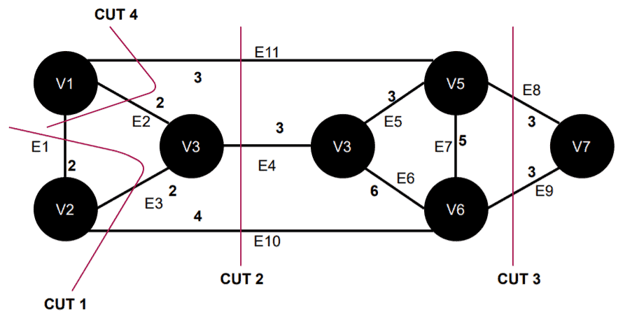
Here in this graph, $CUT \ 3$ is an example of a minimum cut. It removes the edges $E8$ and $E9$ , and the sum of weights of these two edges are minimum among all other cuts in this graph.

3. Maximum Flow in a Graph

Formally, given a graph $G=(V, X)$ , a flow in $G$ is a vector $\phi = (\phi_{1}, \phi_{2}, \phi_{3},...,\phi_{n}) \in R^{P}$ in a way that in every vertex $x_{i} \in X$ , the Kirchhoff law is verified (Law of conservation of flow at nodes). According to Kirchhoff’s law, the sum of the flow entering a node (or a vertex) should be equal to the sum of the flow coming out of it.

Let’s consider this graph:

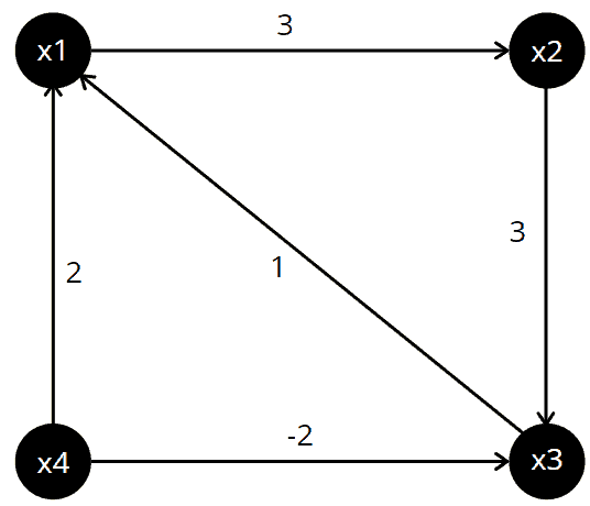
Here all edges represent a flow value, so the set or vector of flows in this graph is $\phi = (3,3,-2,2,1)$ .

These flow values satisfy the Kirchhoff law. For $x_{1}$ , the sum of flows equal to $\mathsf{3}$ for the outgoing edges. Similarly, the sum of flows equal to $1+2=3$ for the incoming edges of $x_1$ , which also equals the previously computed sum. This can be checked for the other vertices.

Flow in a network or a graph follows some properties. In a flow graph, there are two special vertices: source $S$ and sink $P$ . Each edge $(u, v)$ in the flow network has a capacity $C(u, v) \geq 0$ . A flow in a graph $G$ is a function $f: V \times V \rightarrow R$ and it satisfies a capacity constraint: for each edge $(u, v), f(u, v) \leq C(u, v)$ . Net flow in the edges follows skew-symmetric property: $f(u, v) = -f(v, u)$ .

A maximum flow is defined as the maximum amount of flow that the graph or network would allow to flow from the source node to its sink node.

4. Max-Flow Min-Cut Theorem

The max-flow min-cut theorem states that the maximum flow through any network from a given source to a given sink is exactly equal to the minimum sum of a cut. This theorem can be verified using the Ford-Fulkerson algorithm. This algorithm finds the maximum flow of a network or graph.

Let’s define the max-flow min-cut theorem formally. Let $G=(X,A)$ be a flow network, $\phi$ a flow on $G$ . The value of the maximum flow from the source $S$ to the sink $P$ is equal to the capacity of the minimum cut $CT$ separating $S$ and $P$ :

$Max (\phi) = Min (C(CT))$

5. The Ford-Fulkerson Algorithm

5.1. Residual Network and Augmented Path

The Ford-Fulkerson algorithm is based on the three important concepts: the residual network augmented path and cut. We already discussed cut in a graph.

A residual network can be defined as $G_f (V,E_f )$ , where $E_f = {(u,v ) \in V \times V : c_f (u,v ) > 0}$ . Residual capacity is defined as $c_f(u,v ) = C(u,v ) - f (u,v)$ .

An augmenting path $p$ is a simple path from source node $S$ to sink node $P$ in the residual network $G_f$ .

We also use a Netflow graph in this algorithm in order to show the flow and capacity for each edge in the graph.

5.2. General Idea

The algorithm starts with a workable flow through the graph, and the flow is improved iteratively.

If this flow is maximum, it makes it possible to determine the flow function satisfying this value as well as the minimum cut. If the flow is not maximum, its objective is to highlight an improving path corresponding to this flow.

Initially, the algorithm starts by setting the flow value between the source and sink node to $\mathsf{0}$ . At each iteration, we find an augmented path and increase the flow value. We’ll terminate the algorithm and return the flow value when no more augmented paths can be found.

5.3. Pseudocode

Let’s see the pseudocode of the Ford-Fulkerson algorithm:

6. Example

Initially, we’re taking a directed connected graph, and we’ll run the Ford-Fulkerson algorithm on it. In each step, we pick an augmented path and present the residual graph and Netflow graph:

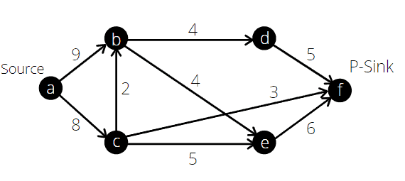
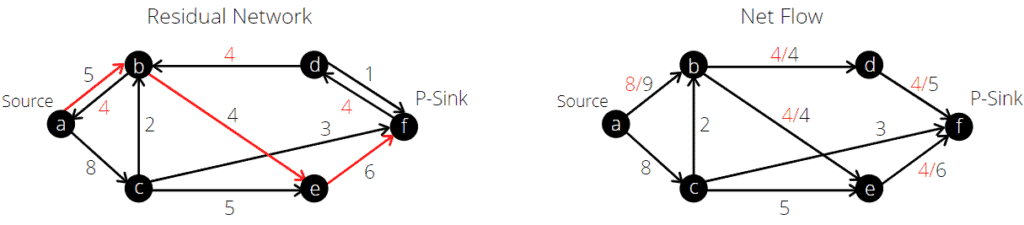
First, we choose the path $a-b-d-f$ . In this path, the minimum capacity is $4$ . Now we’ll construct a residual graph and a Netflow graph:

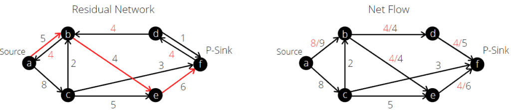
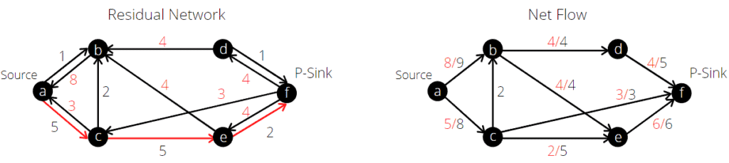
We’ll continue the algorithm and select the next augmented path $a-b-e-f$ :

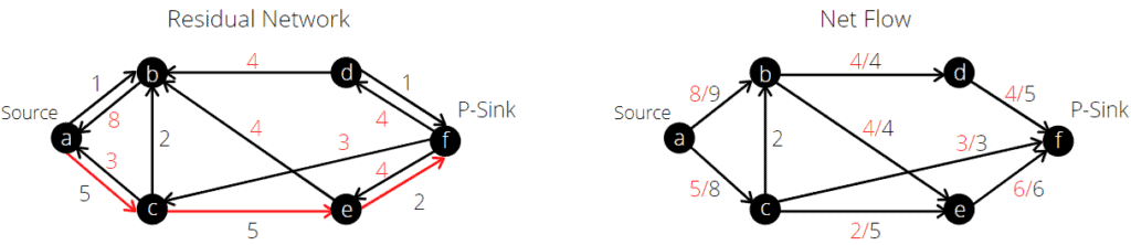
Our next pick is $a-c-f$ :

Still, we can pick more augmented paths. We pick the path $a-c-e-f$ :

Now let’s observe the residual graph, and let’s see if we can find more augmented paths:

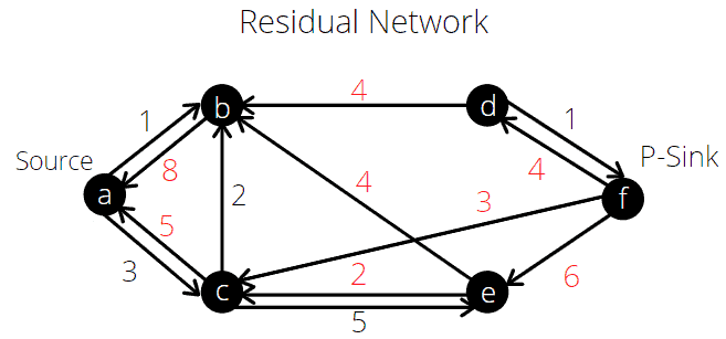
If we see the current residual graph from the source node $a$ , we can’t reach the sink node $f$ via a path. Therefore, we terminate the algorithm as we can’t find any more augmented paths. Now according to the algorithm, the maximum outgoing flow from the sink node should be equal to the maximum incoming flow of the source node. Let’s verify this.

The maximum outgoing flow from the node $\mathbf{f}$ is $\mathbf{13}$ and also the maximum incoming flow for the source node $\mathbf{a}$ is $\mathbf{13}$ , Hence, we verified that the Ford-Fulkerson algorithm works fine and provides the maximum flow of a graph correctly.

Now according to the maximum-flow minimum-cut theorem, the minimum cut of this graph would be equal to the maximum flow of the graph. Therefore, the minimum cut of this example graph is $\mathbf{13}$ .

7. Time Complexity Analysis

The Ford-Fulkerson algorithm depends heavily on the method used to find an augmented path. An augmented path can be found using a Breadth-first search (BFS) or Depth-first search (DFS). If we choose an augmented path using BFS or DFS, the algorithm runs in polynomial time.

The execution time of BFS is equal to $\mathcal{O}(E')$ , where $E'$ is the number of edges in the residual graph $G_f$ . For each edge, the flow will be increased, and in the worst case, it reaches its maximum flow value $f^{*}$ . Therefore the algorithm will be iterated at most $f^{*}$ times. Hence, the overall time complexity of the Ford-Fulkerson algorithm would be $\mathbf{\mathcal{O}(f^{*} \times E')}$ .

8. Conclusion

In this tutorial, we discussed how to find a minimum cut by calculating the maximum flow value of a graph. We presented the Ford-Fulkerson algorithm to solve the maximum flow problem in a graph.

To find the minimum cut of a graph, we discuss the max-flow min-cut theorem. Finally, we verified the Ford-Fulkerson algorithm with an example and analyzed the time complexity.

Full Archive

About Baeldung

Core Concepts

Operating Systems

Artificial Intelligence

Graph Theory

Latex