In-Place Sorting With Merge Sort | Baeldung on Computer Science

1. Overview

Merge sort is one of the fastest sorting algorithms. However, it uses an extra buffer array while performing the sort. In this tutorial, we’ll implement an in-place merge sort algorithm with constant space complexity.

Initially, we’ll quickly remind you of the traditional merge sort algorithm. After that, we’ll give two approaches to implementing an in-place version of the algorithm. Finally, we’ll provide a step-by-step example to show how the algorithm performs the sorting.

2. Traditional Merge Sort

In the traditional merge sort algorithm, we use an additional array to merge sorted parts. Let’s start by giving an example of how the algorithm works and then discuss the time and space complexities.

2.1. Example

The merge sort algorithm divides the array in half, sorts each recursively, and then merges the two sorted parts. To merge the two parts, we use an auxiliary array called the buffer array. Let’s check the following example:

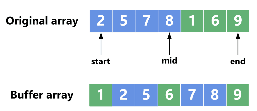
After sorting the two halves of the original array, we merged both parts into the buffer array. This is done by taking the smaller element between both halves and appending it to the buffer array. After this is done, the content of the buffer array can be copied over to the original array.

2.2. Complexity

The time complexity of merge sort is $O(n \cdot log(n))$ , where $n$ is the number of elements inside the array. Although the time complexity is considered very good, the space complexity is a problem. Since we need the buffer array to merge the sorted parts, the space complexity of merge sort is $\mathbf{O(n)}$ , where $\mathbf{n}$ is the size of the array.

3. Naive In-Place Merge Sort

Let’s start with the naive approach to implementing an in-place merge sort. We’ll provide an example, then jump into the implementation and discuss the complexities of time and space.

3.1. Naive Approach Example

Since we’ll use an in-place approach, we can’t define any buffer arrays and must perform the merge sort on the same array. To merge two sorted parts of the array, we always compare the smaller element in each part and output the smaller one to the result.

Note that when using the same array to perform the merge, and if the element on the left part is smaller than the element on the right, we don’t need to do anything. This is because the element on the left side is already in its correct location.

However, if the element on the right is smaller, it must be placed before all the elements on the left side. Therefore, we’ll shift the elements on the left side to the right by one, freeing one space before it. Then, we can move the small element into that space.

This can be shown through the following example:

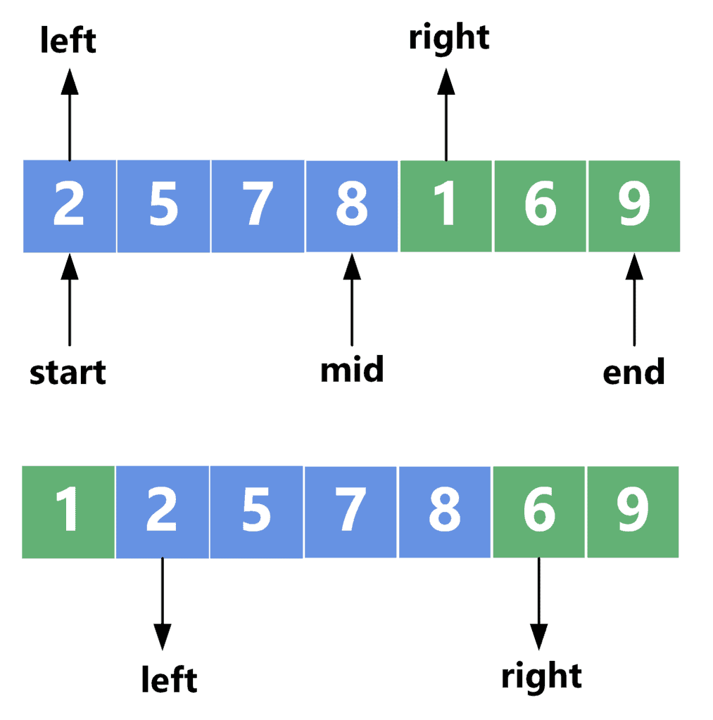
As we can see, the values $left$ and $right$ point to the first element in each part. Since $array[right] = 1$ is smaller than $array[left] = 2$ , we shift all the elements on the left side one step forward. After that, we place the smallest value in its place and move the $right$ pointer one step forward to the next element.

Now, we can move to implement the algorithm described in this example.

3.2. Naive Approach Implementation

Take a look at the implementation of the naive approach:

We define a function called $naiveMergeSort$ that takes the required array and the $start$ and $end$ positions of the array. Initially, this function should be called with $start = 0$ and $end = n - 1$ , where $n$ is the size of the array.

We start by checking the base case. If we reach an array with a size of less than one, then this array is already sorted, and we return immediately. Otherwise, we sort both halves recursively.

Once both halves are sorted, we start the merging process. We check if the left element is smaller than the right one. If so, then it’s already in its correct place. Thus, we only move the $left$ pointer one step forward to the next element.

However, if the right element is smaller, we shift the array’s left part one step forward and place the right element before the left part. After that, we move the $left$ , $mid$ , and $right$ pointers one step forward.

After the $while$ loop ends, it means one of the two conditions was broken. If $left$ reaches the $mid$ point, all the left-side elements are already in place, and whatever is left to the right is already in the correct place.

If the $right$ pointer reached the end, we already placed all right-side elements in their correct place. In this case, the left-side elements remain at the end of the array, which should already be in their correct place.

3.3. Naive Approach Complexity

The extra space complexity of the naive approach is $\mathbf{O(1)}$ because we didn’t use any additional arrays besides the original one. However, the time complexity is a little tricky to calculate. To do that, take a look at the following figure:

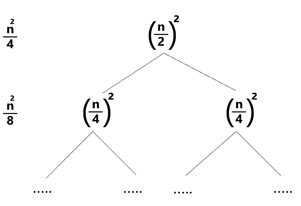
The first level represents the merging that is done on the full array. At that level, the array is divided into two halves. In the worst case, we’ll shift the right part $n/2$ times, where $n$ is the number of elements. Each shifting operation takes approximately $n/2$ operations. Thus, the overall complexity for that level is $O(n^2/4)$ .

The next level is applied twice, one time for each half. Similarly to the previous case, we need $n/4$ shifting operations for each half that result in a total of $n^2/16$ complexity. However, since this is applied on each half, the overall complexity is $O(2 \cdot n^2/16)$ , which is $O(n^2/8$ ).

By following this sequence, we can formulate the following formula for the time complexity:

$complexity = \dfrac{n^2}{4} + \dfrac{n^2}{8} + ...$

$complexity = \sum_{i=2}^{log(n)} \dfrac{n^2}{2^i}$

$complexity = \dfrac{n^2}{2}$

As a result, we can see that the overall time complexity is $\mathbf{O(n^2)}$ , where $\mathbf{n}$ is the size of the array.

4. Advanced In-Place Approach

We’ll start by explaining the theoretical idea behind the advanced approach. After that, we can implement the algorithm and provide an example to explain it.

4.1. Theoretical Idea

Since we don’t want to use any buffer arrays, we’ll need to use parts of the original array to merge sorted parts. To achieve this, the buffer array inside the original array must satisfy one of the following two conditions:

The size of the two sorted parts must not exceed the size of the buffer area.
The buffer area can overlap with one of the sorted parts. However, we must ensure that none of the unsorted elements gets overwritten.

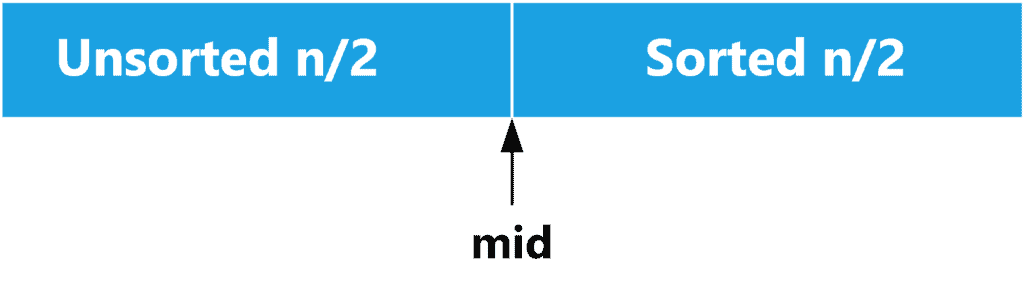
Let’s say we want to sort the full array. We can recursively sort the right part of the array. We will end up with a case like the following:

However, we can’t recursively sort the left part of the array because we will have two sorted parts and no buffer area to merge them. Nevertheless, we can divide the left part into two halves, and sort the first one recursively. After that, we come to the following scenario:

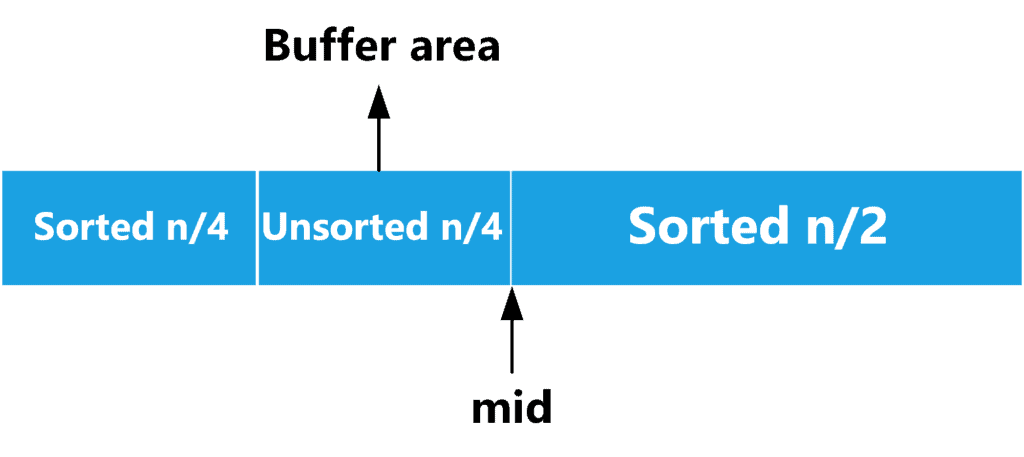
The idea here is that we want to merge the two sorted parts using the remaining unsorted part as the buffer area. The unsorted part forms one-quarter of the elements and, therefore, doesn’t satisfy the first condition for the buffer area.

However, let’s take a closer look at the merging process. If the element on the left-sorted part is smaller, then we can replace it with the element from the buffer area. Since the first sorted part also forms one-quarter of the elements, the elements should fit into the buffer area.

If the right sorted part is smaller, we will replace it with the element from the buffer area. However, this means the buffer area lost one place from its beginning and gained one new place at the end. Thus, its capacity remained untouched. Therefore, we can always ensure that no elements will be overwritten and end up with the following result:

Finally, following the same approach, we can keep reducing the buffer area size by half. If we reach the base case of two elements, we can use insertion sort, for example, to sort them.

Now, let’s implement the above-mentioned approach.

4.2. Merge Function

We’ll dive into the implementation step by step. First, let’s implement the merge function:

We define the function $merge$ that takes the original array, the first range $[from1, to1]$ , the second range $[from2, to2]$ , and the beginning of the buffer area. We keep comparing the first element from each range since it’s the smallest one. We move the smallest one to the buffer area and replace it with the element there. We also advance the corresponding pointers one step forward.

When the $while$ loop breaks, it means only one of the two ranges ended. Therefore, we similarly copy the remaining part of the other range to the buffer area.

4.3. In-Place Merge Sort Implementation

After defining the merge function, we can now define the sort algorithm. Take a look at the implementation:

We define two functions. The first one is $sortWithBuffer$ which sorts the range $[from, end]$ and writes the result to the buffer area starting at pointer $buffer$ . We start with the base case. If we only have one element, we move that element to the buffer.

Otherwise, we divide the array in half, recursively sort each part using the $mergeSort$ function, and then merge both parts into the buffer area using the $merge$ function defined in section 4.3.

The second function is $mergeSort$ , the main function that sorts the array. We start by dividing the array in half, sorting the first part, and writing the result to the buffer area, which is the second part. Note that if the array’s length is odd, then we make sure to choose the $mid$ so that the sorted part can fit into the buffer area.

Now, we’ve divided our array into a range $[L_1, R_1]$ forming the unsorted part, and $[L_2, R_2]$ forming the sorted part. Next, we’ll keep reducing the size of the unsorted part until it becomes very small that we can use insertion sort to merge it with the sorted part.

Therefore, we’ll divide the unsorted part into two halves, sort the second part, and write the result in the first part. Note that we pay attention to defining the $mid$ in a way that keeps the buffer area big enough to hold the sorted elements.

After that, we merge the sorted part at the beginning of the array with the sorted part at the end and write the result into the buffer area in the middle of the array, as explained in section 4.1. Once this is done, we’ll have the sorted part at the end of the array, while the unsorted part remains at the beginning. We keep repeating this process until the size of the unsorted part becomes two elements.

Finally, we perform insertion sort to place the remaining two elements at their correct location in the sorted part.

4.4. Time and Space Complexity

The additional space complexity is $\mathbf{O(1)}$ because we didn’t use any extra arrays. This approach is similar to the original merge sort approach regarding the time complexity. We only manipulate the location of the buffer area, which replaces the auxiliary array we used in the original approach.

The only difference is the insertion sort we perform at the end, which is $O(n)$ . However, this is done at each level of the recursion. In total, we have $O(log(n))$ levels because we keep dividing the array in half. Therefore, its complexity is $O(n \cdot log(n))$ . This step is performed after the recursion. Thus, its complexity is added to the overall complexity.

As a result, the overall time complexity is $\mathbf{O(n \cdot log(n))}$ .

4.5. Example

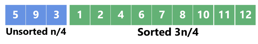
Let’s provide a step-by-step example of how the $merge$ function works. Take a look at the following array:

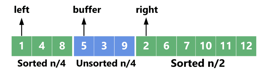
The first quarter is sorted, the second one is the buffer area, and the second half is sorted. We start by comparing the first element in each sorted part and moving the smallest to the buffer area. In this case, $array[left] = 1$ is smaller than $array[right] = 2$ . Thus, we swap it with the first element in the buffer area:

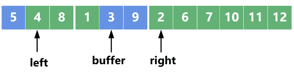
Next, we compare $array[left] = 4$ with $array[right] = 2$ . Since the element on the right is smaller, we swap it with the next element in the buffer area:

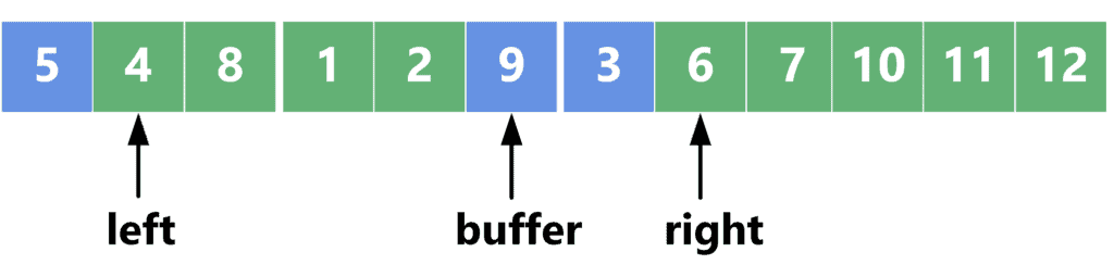
Note that element 3 from the buffer area seems to be added to the second sorted part. However, this is not correct. Actually, the right sorted part now starts at the position of the $right$ , while the buffer area contains ${9, 3}$ . We also have element $5$ at the beginning of the array.

After the $merge$ function ends, we’ll get the following array:

As we can see, the first quarter of the array contains unsorted elements in a different order than they originally appeared. This shouldn’t matter since they are unsorted anyways. The other part of the array now contains sorted elements.

5. Conclusion

In this tutorial, we discussed the in-place merge sort. We started with a quick reminder of how merge sort works, then presented two approaches to writing the in-place implementation. We also provided a step-by-step example of how the merge function works.

Full Archive

About Baeldung

Core Concepts

Operating Systems

Artificial Intelligence

Graph Theory

Latex