

Yes, we're now running our only Summer Sale. All Courses are 30% off until 20th July, 2026:
Learn through the super-clean Baeldung Pro experience:
>> Membership and Baeldung Pro.
No ads, dark-mode and 6 months free of IntelliJ Idea Ultimate to start with.
1. Overview
In this tutorial, we’ll take a closer look at the divide and conquer-based efficient sorting algorithm known as Merge sort. To begin, we’ll examine two distinct Merge Sort approaches, top-down and bottom-up in-depth, both of which are vital.
Later, we’ll go over the implementation of bottom-up and top-down approaches and how they work. To summarize, we’ll show how to use specific merge sort algorithms using simple examples, as well as their time and space complexity.
2. Top-Down Approach
As the name implies, this approach begins at the top of the array tree and works its way down. Consequently, halving the array, making a recursive call, and merging the results until it reaches the bottom of the array tree. The term “recursive approach” also applies to the top-down merge sort method.
Top-down merge sort begins with an array of inputs. It divides the input array in half. Further, it calls merge sort recursively on the array’s halves. Finally, we merge the array halves into a final result array, which returns the merged output array.
This recursive method’s base case is if the length of the array to sort is indivisible into two, in which case no recursive call to sort or merge the array halves is required.
To better understand how Top-down merge sort works, consider the example shown below:
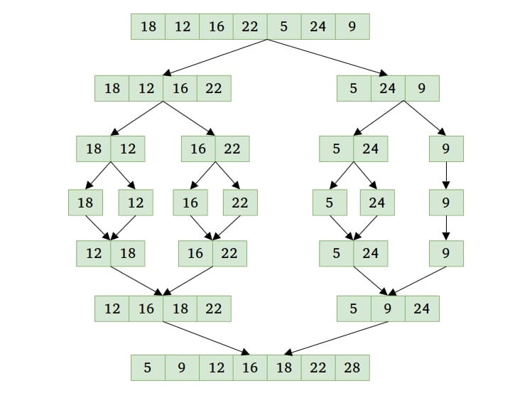
In fact, the merge sort divides an array into subarrays and merges them recursively. Furthermore, the dividing process is repeated until a sub-sequence with a single item is obtained.
Afterward, a single-item sequence is easily sorted. The entire process is finished during the merge stage, which joins two sorted lists to create a single array with sorted items. The merging process turns out to be quite simple to put into action.
In a nutshell, recursion is a method employed in the top-down merge sort approach. As it descends from the top of the tree, it divides the array in half, makes recursive calls, and merges the outcomes until it reaches the bottom.
2.1. Top-Down Merge Sort Algorithm
The following basic phases are followed in a Merge sort algorithm on an input sequence  with
with  elements:
- Step 1: divide into two sub-sequences of approximately
 elements each
 - Step 2: By calling recursively, sort each subsequence
- Step 3: Combine the two sorted sub-sequences or sub-array into a mono-sorted array
Pseudocode for the Top-down approach merge sort algorithm:
algorithm TopDownMergeSort(S):
    // INPUT
    //     S = sequence with n elements
    // OUTPUT
    //     sorted sequence S

    if S.size > 1:
        (S1, S2) <- partition(S, n/2)
        TopDownMergeSort(S1)
        TopDownMergeSort(S2)
        S <- merge(S1, S2)
2.2. Time and Space Complexity
Merge Sort always divides the array into two halves, and it takes linear time to merge the two halves, so its time complexity is  .
.
When merging two sorted arrays into a single array, we need space to store the merged result.
We’ll need  space in total because the arrays we’ll be combining have items. However, because we’re using recursion calls and this additional array will be copied
  times, the space complexity, in this case, is
  .
.
3. Bottom-Up Approach
The bottom-up (non-recursive) method merges each subsequent pair of items into sorted passes of length two. Next, we combine these into more sorted runs of length four. And after that, merge those into sorted passes of length eight, and so on. We merge until it returns a sorted array containing all input array elements.
Consider the following example to understand better how bottom-up merge sort works:
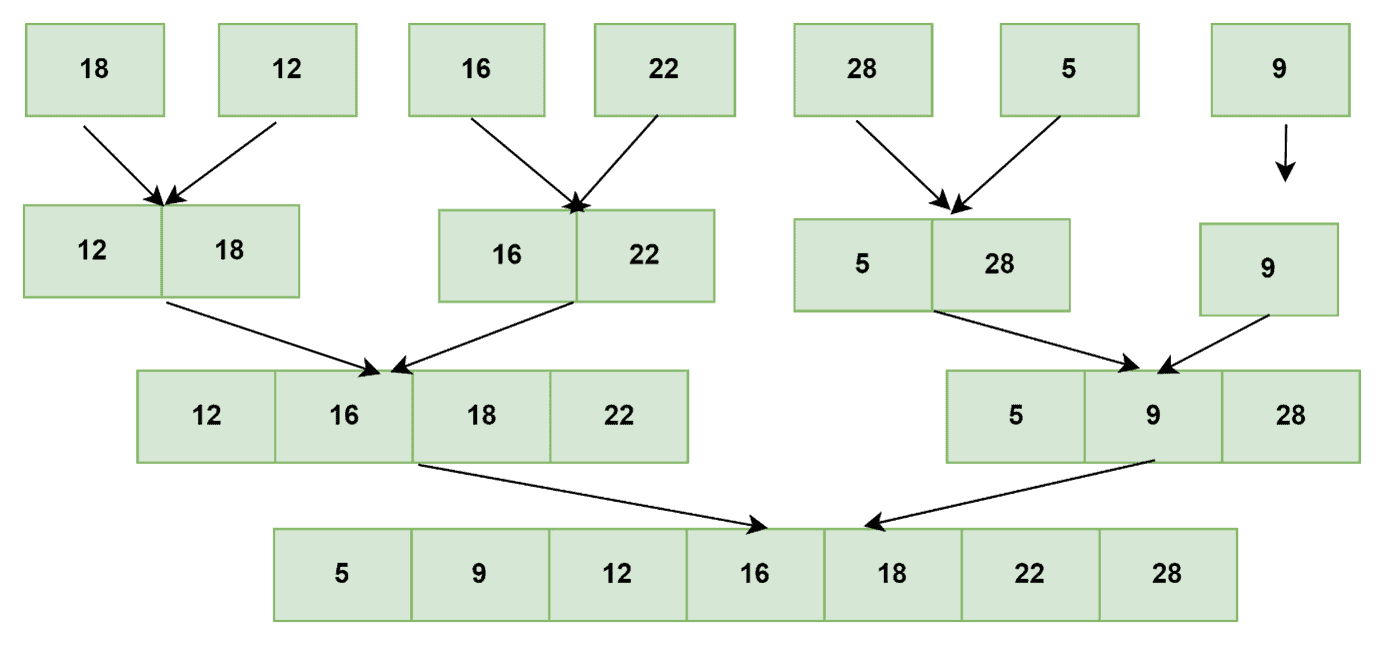
The Bottom-Up merge sort method employs the iterative technique. It starts with a single-element array and then merges and sorts two nearby items. The merged arrays are merged and sorted again until there is only one unit of the sorted array left. In other words, recursion is not used in the bottom-up implementation. It starts at the bottom of the tree and works its way up by iterating over the pieces and merging them.
3.1. Bottom-Up Merge Sort Algorithm
Pseudocode for the Bottom-UP approach merge sort algorithm:
algorithm BottomUpMergeSort(S, n):
    // INPUT
    //     S = sequence with n elements
    // OUTPUT
    //     sorted sequence S

    if n < 2:
        return
    i <- 1
    while i < n:
        j <- 0
        while j < n - i:
            if n < j + i * 2:
                merge(A + j, A + j + i, A + n)
            else:
                merge(A + j, A + j + i, A + j + i * 2)
            j += i * 2
        i = i * 2
3.2. Time and Space Complexity
As we perform merges for  passes, the time complexity is , and the space complexity is
  due to the use of an auxiliary array in the merge routine. We reduced the space complexity in this version, making it superior to the recursive one.
4. Conclusion
This article discussed one of the most widely used sorting algorithms, merge sort. We went over the two merge sort approaches in depth. To better understand their implementation, we explain top-down and bottom-up approaches with examples and algorithms.
Finally, we presented the time and space complexity of both approaches. As a result, readers will have a clear grasp of merge sort approaches and their potential applications.