What Are the Advantages of Kernel PCA Over Standard PCA?

1. Introduction

In this tutorial, we’ll explain the benefits of incorporating kernels in the context of Principal Component Analysis (PCA). Firstly, we’ll provide a concise overview of the PCA technique. Following that, we’ll delve into the concept of kernel PCA, outlining its characteristics and enumerating the advantages it offers.

Finally, we’ll present various practical applications where kernel PCA proves its efficacy.

2. What Is PCA?

Principal Component Analysis (PCA) is a widely used statistical method and dimensionality reduction technique in data analysis and machine learning. The main goal of PCA is to simplify high-dimensional datasets while retaining essential information. PCA achieves it by transforming the original data into a new coordinated system, where the data variance is maximized along the new axes. Those axes represent principal components.

For example, we can take a two-dimensional data set, represented with blue dots in the image below. There are two ways of finding the principal components:

• Maximum variance – finding the first principal component, such that the variance of the orthogonal projection of the data into a lower-dimensional linear space, defined by that component, is maximized.
• Minimum Error – finding the first principal component, such that the mean squared error of distances between data points and their projections is minimally possible. In the image below, those distances are red lines.

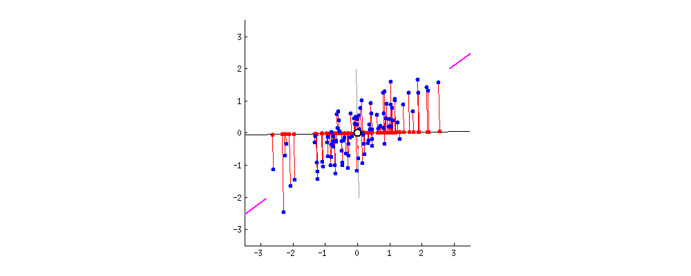
Every subsequent principal component needs to be orthogonal to the previous principal components. Also, we can find it in the same way as the previous ones. Notice that PCA doesn’t reduce data dimension directly but finds new axes for the data. In essence, PCA tries to find a different view of the data in which we can separate it better:

Then, PCA finds principal components from the most useful to the least useful. This usefulness is defined with an explained variance ratio. If we want to reduce the dimensionality of the data, we’ll take top N principal components. An effective approach is determining the number of dimensions where the cumulative explained variance surpasses a specified threshold, such as 0.95 (or 95%).

3. What Is Kernel PCA?

While traditional PCA is highly effective for linear data transformations, it may not capture the underlying structure of complex, nonlinear datasets. To handle this problem, we introduce kernel principal component analysis (KPCA). KPCA relies on the intuition that many data sets that are not linearly separable in their current dimension can be linearly separable by projecting them into a higher-dimension space.

In one sentence, KPCA takes our data set, maps it into some higher dimension, and then performs PCA in that new dimensional space.

To gain a better intuition of this process, let’s examine the following example:

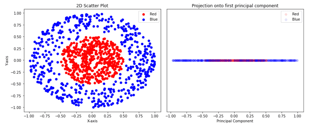
On the left side, we have our two-dimensional data set. This data set consists of two classes; red and blue. Blue classes are points on a donut-shaped cluster, while red points are in the circle that is in the centre of that donut. It’s clear that this data set is not linearly separable, which means that no straight line can separate these two classes.

If we apply PCA and reduce our data dimension from 2D to 1D, we’ll get points on the one axis in the image right. The goal of PCA is to simplify high-dimensional datasets while retaining essential information. But, as we can see in the right figure, points are now mixed, and we cannot separate or cluster them.

Now, let’s transform our data set from 2D to 3D with a simple function

(1)  

where is a point in 2D space. Visually, this transformation looks like this:

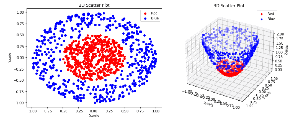
Following the logic of KPCA, we transformed our data set to a higher dimension, from 2D to 3D. Now we can try to apply PCA and reduce the dimensionality from 3D to 1D. Moreover, let’s transform our data firstly to 2D and after to 1D. The results are below:

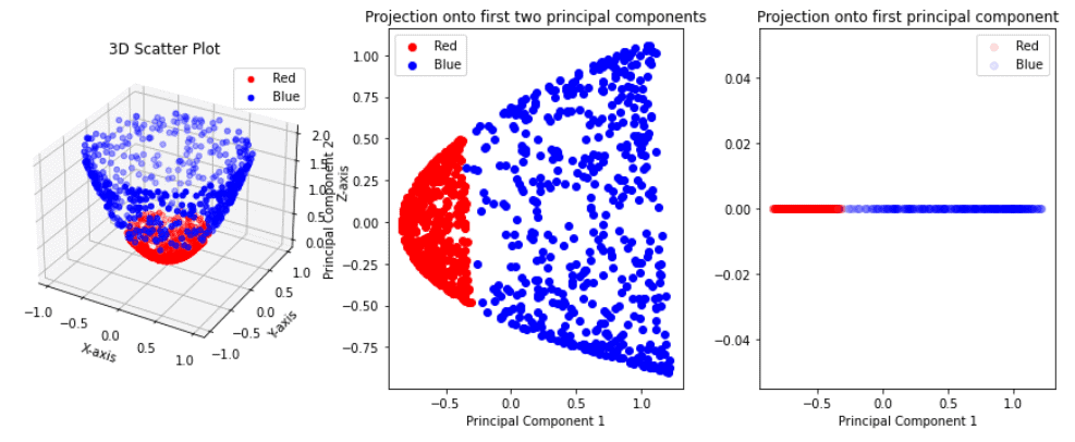
Unlike the initial attempt, the projection onto the first principal component now effectively separates the red and blue points. This outcome highlights the true potential of Kernel PCA over the standard PCA.

3.1. Kernel Functions

Kernel function is a function that we use to transform the original data into a higher-dimensional space where it becomes linearly separable. Generally, kernels are commonly employed in various machine learning models such as support vector machines (SVM), kernel ridge regression (KRR), kernelized k-means, and others. Some of the most popular kernel functions are:

• Linear: ,
• Polynomial: ,
• GaussRBF: ,
• Sigmoid:

Usually, it’s not easy to determine which kernel is better to use. One good option is to treat the kernel and its parameters as hyperparameters of the whole model and apply cross-validation to find them together with other hyperparameters.

Transforming the data into a higher dimension directly can be a very costly operation. To overcome the explicit calculation of that transformation, we can use the kernel trick. It’s a machine learning technique to map data into a higher-dimensional space implicitly.

4. Kernel PCA VS Standard PCA

Kernel PCA and standard PCA each have their own set of advantages. Here we’ll mention some of them.

4.1. Advantages of Kernel PCA

Some of the advantages of kernel PCA are:

• Higher-dimensional transformation – by mapping data into a higher-dimensional space, kernel PCA can create a more expressive representation, potentially leading to better separation of classes or clusters
• Nonlinear transformation – it has the ability to capture complex and nonlinear relationships
• Flexibility – by capturing nonlinear patterns, it’s more flexible and adaptable to various data types. Thus, kernel PCA is used for many domains, including image recognition and speech processing

4.2. Advantages of Standard PCA

Some of the advantages of standard PCA are:

• Computational efficiency – standard PCA is computationally more efficient than Kernel PCA, especially for high-dimensional datasets
• Interpretability – it’s easier to understand and interpret the transformed data
• Linearity – excels in capturing linear patterns

5. Applications of Kernel PCA

Kernel PCA finds applications in various fields where nonlinear data relationships must be captured. Some notable applications of kernel PCA include:

• Image Recognition – kernel PCA can effectively capture the nonlinear patterns in image data, making it valuable in image recognition tasks. Some examples are facial recognition systems and object detection
• Natural language processing (NLP) can be applied to analyze and reduce the dimensionality of textual data for tasks such as text classification, sentiment analysis, and document clustering
• Genomics and bioinformatics – in genomics, kernel PCA can help analyse gene expression data, DNA sequencing data, and protein structure data, where nonlinear relationships often exist
• Finance-kernel PCA is used in financial modelling to capture complex, nonlinear relationships in stock price movements and financial data

6. Conclusion

In this article, we’ve explained kernel PCA. Also, we’ve presented the intuition behind it, and the advantages of kernel PCA and standard PCA and explored some of its applications.

Kernel PCA is a powerful technique for uncovering hidden non-linear features within complex data, particularly when combined with other machine learning methods. It can be highly valuable in the creation of new features for data preparation.