What Is Independent Component Analysis (ICA)? | Baeldung on Computer Science

1. Intro

In this tutorial, we’ll explain what is independent component analysis (ICA). This is a powerful statistical technique that we can use in signal processing and machine learning to filter signals. Besides the explanation of the ICA concept, we’ll show a simple example of the problem that ICA solves.

2. Cocktail Party Problem

The simplest way to understand the ICA technique and its applications is to explain one problem called the “cocktail party problem”. In its simplest form, let’s imagine that two people have a conversation at a cocktail party. Let’s assume that there are two microphones near both people. Microphones record both people as they are talking but at different volumes because of the distance between them. In addition to that, microphones record all noise from the crowded party. The question arises, how we can separate two voices from noisy recordings and is it even possible?

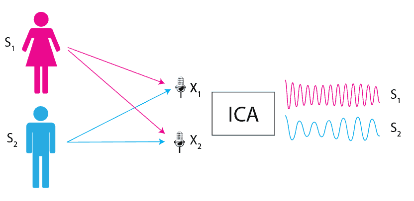
3. Independent Component Analysis Definition

One technique that can solve the cocktail party problem is ICA. Independent component analysis (ICA) is a statistical method for separating a multivariate signal into additive subcomponents. It converts a set of vectors into a maximally independent set.

Following the image above, we can define the measured signals $X_{i}$ as a linear combination:

(1) $\begin{align*} X_{i} = a_{i1}S_{1} + a_{i2}S_{2} =\sum_{j}{a_{ij}S_{j}}, \end{align*}$

where $S_{j}$ are independent components or sources and $a_{ij}$ are some weights. Similarly, we can express sources $S_{i}$ as a linear combination of signals $X_{i}$ :

(2) $\begin{align*} S_{i} = \sum_{j}{w_{ij}X_{j}}, \end{align*}$

where $w_{ij}$ are weights.

Using matrix notation, source signals $S$ would be equal to $S = WX$ where $W$ is a weight matrix, and X are measured signals. Values from $X$ are something that we already have and the goal is to find a matrix $W$ such that source signals $S_{i}$ are maximally independent. Maximal independence means that we need to:

Minimize mutual information between independent components or
Maximize non-Gaussianity between independent components

3.1. Assumptions for Independent Component Analysis

To successfully apply ICA, we need to make three assumptions:

Each measured signal is a linear combination of the sources
The source signals are statistically independent of each other
The values in each source signal have non-Gaussian distribution

Two signals $x$ and $y$ are statistically independent of each other if their joint distribution $p(x, y)$ is equal to the product of their individual probability distributions $p(x)$ and $p(y)$ :

(3) $\begin{align*} p(x, y) = p(x)p(y). \end{align*}$

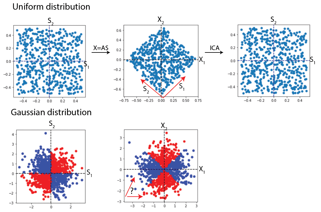
From the central limit theorem, a linear combination between two random variables will be more Gaussian than either individual variable. If our source signals are Gaussian, their linear combination will be even more Gaussian. The Gaussian distribution is rotationally symmetric, and we wouldn’t have enough information to recover the directions corresponding to original sources. Hence, we need the assumption that the source signal has non-Gaussian distribution:

4. Independent Component Analysis Algorithms

To estimate one of the source signals, we’ll consider a linear combination of $X_{i}$ signals. Let’s denote that estimation with $y$ :

(4) $\begin{align*} y = w^{T}X, \end{align*}$

where $w$ is a weight vector. Next, if we define $z = A^{T}w$ we have that:

(5) $\begin{align*} y = w^{T}X = w^{T}AS = z^{T}S. \end{align*}$

From the central limit theorem, $z^{T}S$ is more Gaussian than any of the $S_{i}$ and it’s least Gaussian if it’s equal to one of the $S_{i}$ . It means that maximizing the non-Gaussianity of $w^{T}X$ will give us one of the independent components.

One measurement of non-Gaussianity can be kurtosis. Kurtosis measures a distribution’s “peakedness” or “flatness” relative to a Gaussian distribution. When kurtosis is equal to zero, the distribution is Gaussian. For positive kurtosis, the distribution is “spiky” and for negative, the distribution is “flat”.

To maximize the non-Gaussianity of $w^{T}X$ we can maximize the absolute value of kurtosis

(6) $\begin{align*} \max |kurt(w^{T}X)|. \end{align*}$

To do that, we can use the FastICA algorithm. FastICA is an iterative algorithm that uses a non-linear optimization technique to find the independent components. Before applying this algorithm, we need to do centering and whitening the input data. It ensures that the mixed signals have zero means and that the covariance matrix is close to the identity matrix.

There are several other algorithms for solving ICA:

Infomax – maximizes the mutual information between the mixed signals and the estimated independent components
The joint approximated diagonalization of eigenmatrices (JADE) – separates mixed signals into source signals by exploiting fourth-order moments
Particle swarm optimization (PSO) – heuristic optimization algorithm that searches the mixing matrix that separates the mixed signals into independent components

5. Applications of Independent Component Analysis

ICA has a wide range of applications in various fields, including:

Signal processing for speech, audio, or image separation. We can use it to separate signals from different sources that are mixed together
Neuroscience – to separate neural signals into independent components that correspond to different sources of activity in the brain
Finance – with ICA is possible to identify some hidden features in financial time series that might be useful for forecasting
Data mining – it’s possible to find patterns and correlations in large datasets

6. Conclusion

In this article, we described the ICA technique by providing a simple example of the problem it solves. We also presented a mathematical definition and explained important terms that we used. ICA is a powerful technique that might be very useful in signal analysis and can uncover hidden patterns.

Full Archive

About Baeldung

Core Concepts

Operating Systems

Artificial Intelligence

Graph Theory

Latex