An Introduction to the Hidden Markov Model | Baeldung on Computer Science

1. Introduction

In this tutorial, we’ll look into the Hidden Markov Model, or HMM for short. This is a type of statistical model that has been around for quite a while. Since its appearance in the literature in the 1960s it has been battle-tested through applications in a variety of scientific fields and is still a widely preferred way to tackle many data modeling tasks up to this day.

The HMM was first used for speech recognition, but since then scientists have used the approach for part-of-speech tagging, time-series analysis, gene prediction, transport optimization, and many other sequence-related tasks. One might wonder, why is the HMM so versatile and effective?

2. The Model

The answer lies both in the solid mathematical principles that the model is based on and the simplicity that comes along with them. Every Hidden Markov Model relies on the assumption that the events we observe depend on some internal factors or states, which are not directly observable. This trait is very general which makes it very applicable and is also where the hidden part of the name comes from.

The Markov part, however, comes from how we model the changes of the above-mentioned hidden states through time. We use the Markov property, a strong assumption that the process of generating the observations is memoryless, meaning the next hidden state depends only on the current hidden state. This consequently also makes things a lot easier to work with mathematically as we’ll see later.

2.1. A Guessing Game

To better understand the characteristics of the Hidden Markov Model let’s start with a classical example process. Consider that there are two close friends, Alice and Bob, which live far away from each other but talk over the phone every day and discuss what they did. They decide to play a guessing game where Alice would try to guess the weather, based only on what Bob told her he was doing that day.

For simplicity, let’s imagine Bob’s behavior is pretty limited. He can do one of three things during the day – walk in the park, go shopping or clean his apartment. Additionally, his actions fully depend on the weather of the given day. The weather will also have only two states – “rainy” or “sunny”.

2.2. The Markov Property

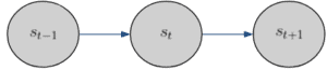
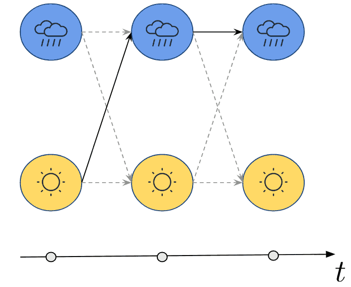
Even with those conditions, it’s still hard to guess, however, we can reason about how Alice might go and tackle this problem. Let’s say that the weather today is exclusively only affected by the weather yesterday. This is the Markov property we already mentioned, an important assumption we are making when using the Hidden Markov Model. Mathematically, we can say the probability of the weather being in a certain state $s$ at a certain time $t$ only depends on time step $t-1$ :

$p(s_{t+1}\mid s_t,s_{t-1}) = p(s_{t+1} \mid s_t)$

This can also be illustrated with a simple diagram with respect to time:

2.3. Markov Chains

Since Alice has an idea of the weather in Bob’s area we can also translate her knowledge into probabilities:

If yesterday was sunny there is a $0.6$ probability that today is sunny again and a $0.4$ probability that it’ll rain. Likewise, if yesterday was raining there is a $0.7$ probability that it rains again and a $0.3$ probability that it is sunny. And since the sequence has to start from somewhere she says that there is a $0.6$ probability of starting with a rainy day and $0.4$ for starting with a sunny day. Alice’s model would then looks like this:

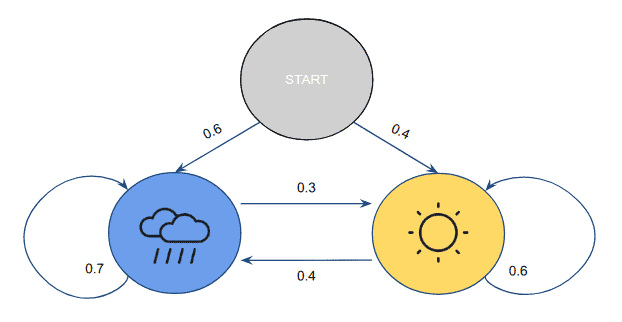
This kind of model is also known as a Markov Chain and the probabilities of getting from one state to the other are called transition probabilities. Generally, these probabilities are defined using a transition matrix. In our example the transition matrix would be: $A = [\begin{matrix} a_{11} & a_{12} & a_{13} \\ a_{21} & a_{22} & a_{23} \\ a_{31} & a_{32} & a_{33} \end{matrix}]$

$A = \begin{bmatrix} a_{11} & a_{12} \\ a_{21} & a_{22} \\ \end{bmatrix} = \begin{bmatrix} 0.6 & 0.4 \\ 0.3 & 0.7 \\ \end{bmatrix}$

One important property to notice, when there is a transition to another state, is that the sum of all transition probabilities given the current state should be 1, or in other words, the rows of our matrix should sum up to one.

And since we got to start from somewhere we define another one-dimensional vector $\pi$ that contains the initial probabilities:

$\pi=\begin{bmatrix} 0.4 & 0.6\end{bmatrix}$

2.3. Model Summary

To sum up, we have some hidden states, let’s call them $N$ , the transition probability matrix $A$ , and the initial probability vector $\pi$ . However, we’d also need to incorporate Bob’s activities somehow. As we said they depend fully on the weather so we can assign conditional probabilities for each state, which are also named emission probabilities.

For example, it sounds reasonable to say that given that today is sunny, there is a $0.8$ probability that Bob will go for a walk, $0.1$ that he goes shopping, and $0.1$ that we clean his house. Since Alice is talking with him each day, however, she has gathered a sequence of observations of his actions and knows better. Depending on her observations, one possible combination of probabilities might be:

$B = \begin{bmatrix} b_{11} & b_{12} & b_{13}\\ b_{21} & b_{22} & b_{23}\\ \end{bmatrix} = \begin{bmatrix} 0.1 & 0.4 & 0.5\\0.6 & 0.3 & 0.1\\ \end{bmatrix}$

where each row of the matrix $B$ represents a hidden state and each column an activity.

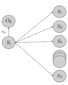
After including $B$ , we now have everything needed to assemble the Hidden Markov Model that gives Alice the best chance of guessing correctly. Visually, we get the following picture:

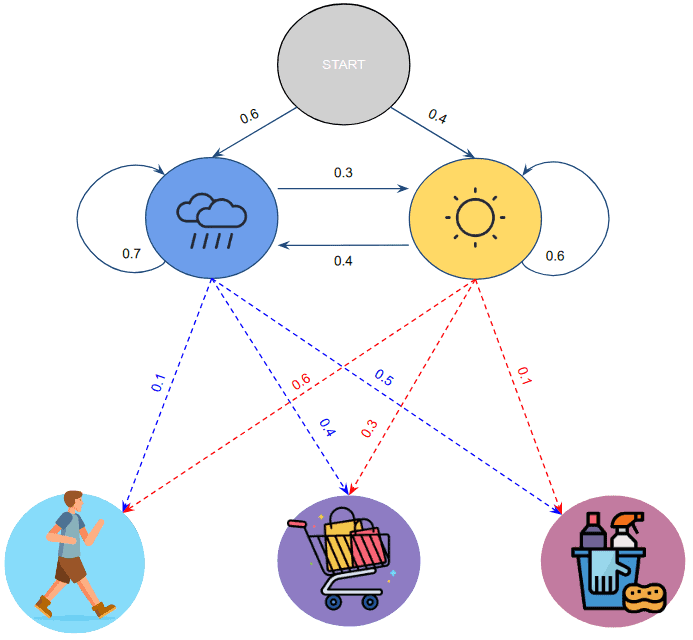
Sure, but how would Alice use it to infer the weather? Well, she’ll need to answer the following question: What is the sequence of hidden states given our model that best explains the given sequence of observations? Answering this, however, is not so trivial.

3. The Evaluation Problem

To better grasp the above question let’s try to answer its inverse first: What is the probability that this particular model generated the given sequence of observations?

Let’s also add some mathematical notation. We have a series of observations $O=\{O_1, O_2,..., O_T\}$ for $T$ time steps, or the number of days talking to Bob in our example. We also have our model in the form of the parameters $A$ , $B$ , and $\pi$ which we can for short denote as $\theta$ . So the question “What is the probability that this particular model generated the given sequence of observations?” can be expressed as:

$p(O_T \mid \theta) = ?$

To answer it, let’s first imagine a particular sequence of hidden states $S$ that generated the sequence of observations. For example, if we have $T=3$ days of observations $O=(Walk, Shopping, Cleaning)$ , one possible hidden sequence might be $S = (Sunny, Sunny, Rainy)$ . What would be the probability of seeing this observation sequence given $S$ ?

We need only to multiply the probabilities of seeing a particular observation $O$ given the hidden state at time $s_t$ :

$p(O_T \mid S_T, \theta) = \prod_{t=1}^{T} p(O_t \mid s_t, \theta)$

This can be easily calculated by looking up the particular emission probability in $B$ for each hidden state in the sequence. For the example $S_3 = (Sunny, Sunny, Rainy)$ this would be:

$p(Walk, Shopping, Cleaning \mid Sunny, Sunny, Rainy)= p(Walk \mid Sunny)* p(Shopping \mid Sunny)* p(Cleaning \mid Rainy) = 0.6 * 0.3 *0.5$

3.1. Formulation

We, however, do not know the exact sequence that gave us the observations. But for starters let’s answer what is the probability of a particular hidden state sequence occurring like the one in our example. Since we are operating under the Markov Property, each state transition is independent and we can again simply multiply:

$p(S \mid \theta) = \prod_{t=1}^{T} p(s_t \mid s_{t-1})$

So, the joint probability of getting a particular hidden sequence $S$ and a particular observation sequence would be:

$p(O,S) = \prod_{t=1}^{T} p(O_t \mid s_t, \theta)\prod_{t=1}^{T} p(s_t \mid s_{t-1})$

We however need to consider all possible combinations of state sequences that could have generated the observation sequence. To do that, we can marginalize out all the joint probabilities of all possible hidden state sequences and them occurring by summation:

$\begin{aligned} p(O \mid \theta) & =\sum_{q=1}^{Q}p(O,S_q \mid \theta) \\ & =\sum_{q=1}^{Q}\prod_{t=1}^{T} p(O_t \mid s_t, \theta)\prod_{t=1}^{T} p(s_t \mid s_{t-1})$

where $Q$ is the number of all possible hidden state sequences.

Calculating this won’t be a problem but the computation complexity is very high for practical scenarios. If the number of hidden states is $N$ there are $N^T$ possible state sequences. For each sequence, we’ll need to multiply $2T-1$ times. And finally, we’ll need to sum them all up for $N^T-1$ operations.

So a total of $(2T-1)N^T + N^T-1$ operations or $O(TN^T)$ in BigO notation.

3.2. The Forward Algorithm

Not all is lost though. In this enormous calculation, there are a lot of redundant products that imply the use of another way of formulating the result we´re after. The most common approach is the Forward-Backward Algorithm which strongly relies on the principles of Divide-and-conquer. As the name suggests this algorithm consists of two parts forward and backward, but only one is usually enough to answer our first question so let’s look at the forward part first.

To employ the forward part of this approach we’ll need to express the probability of a particular hidden state $s_i$ at a particular time $t$ in terms of the time steps before it. We are going to do this inductively, by introducing a new aggregate variable $\alpha$ , which is going to capture the probability of seeing a series of observations up to a certain point $t$ and then end up at $S_i$ given our model:

$\alpha_t(i) = p(O_1,O_2,...,O_3, q_t=S_i \mid \theta)$

The base case for our variable would then be:

$\alpha_1(i) = \pi_i b_i(O_1)$

for $1 \le i\le N$ .

And then for our the inductive step we describe more generally $\alpha_{t+1}$ :

$\alpha_{t+1} = \bigg[\sum_{i=1}^{N}\alpha_t(i) a_{ij}\bigg]b_j(O_{t+1})$

for $1 \le t \le T-1$ and $1 \le i\le N$ .

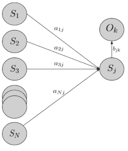
What the above equation is saying is that the probability of seeing the series of observations up to $t$ and ending up at state $j$ is equal to the sum of all the different ways of getting to state $j$ given our observation sequence( $\sum_{i=1}^{N}\alpha_t(i)$ ) multiplied by the probability of actually transitioning to $j$ ( $a_{ij}$ ) and also observing the next observation $O_{t+1}$ given that we are now at state $j$ ( $b_j(O_{t+1})$ ).

Another way to look at the equation is through a diagram

The only thing we need to additionally account for is that in the last time step we don’t need to transition anymore so we can just sum over all alphas:

$p(O_T \mid \theta) = \sum_{i=1}^{N}\alpha_T(i)$

Overall, the algorithm works significantly faster for computing $p(O_T \mid \theta)$ compared to the naive calculation. Since for every time step, we are considering all previous states in the computation for every one of the next states we have a computational complexity of $O(TN^2)$ which is a significant improvement.

3.3. The Backward Algorithm

What is more interesting about the Forward-Backward algorithm, though, is that as the name suggests, it works in reverse. As we have all the observations we can just apply the same logic backward. Instead of defining a parameter for the probability of seeing observations up to a certain point and being in a state $S_i$ , we can define a new recursive parameter $\beta$ that’ll describe the probability of being in state $S_i$ at time $t$ knowing what observations are ahead.

To formulate the base case of $\beta$ we start from the end of our observations. Since there are no other observations following, we define it as one:

$\beta_T(i) = 1$

and that’s for every one of our states $1 \le i \le N$ .

And then inductively we can define every other $\beta$ to be:

$\beta_t(i) = \sum_{j=1}^{N}a_{ij}b_j(O_{t+1})\beta_{t+1}$

In this equation again, just like with $\alpha$ we are considering all possible state transitions between states but instead of accounting for the transitions forward we are looking backward and describing $\beta_t$ not with the one before it, but with the ones after it.

Here is a diagram to highlight the difference:

4. The Decoding Problem

Now we are ready to answer our original question “What is the sequence of hidden states given our model that best explains the given sequence of observations?”.

One way of doing it would be to use our knowledge from the last section and calculate the probability that our model generated the observation we saw for every possible sequence of hidden states and then find the one sequence that has the biggest resulting value. Just like in the last section, however, we’ll find that that’ll be infeasible to calculate with brute force.

What we can do is try to take inspiration from the Forward-Backward Algorithm. In both versions of that algorithm, we´re summing over each hidden sequence of states in a smart recursive way. Why not do something similar, but instead of using the summation operator use the $max$ one. The resulting approach is called the Viterbi algorithm.

Just like before we can define a recursive variable that’ll contain the most probable path up to the current time step $t$ and ends up at state $S_i$ . The base case will start from the first time step and looks like this:

$\delta_1(i) = \pi_i b_i(O_i)$

$\psi_1(i) = 0$

The only thing that is different here is that we need to take note of where we came from at each time step to recreate the path. To this end, we define a variable $\psi$ which would denote what state we came from given that we are at the current state $S_i$ .

For the base case $\psi$ we don’t need to track any state so it’ll simply be equal to zero.

As one might guess, the basic inductive step to extend our new parameters is again similar to the one in the Forward-Backward Algorithm:

$\begin{array}{lr} \delta_{t}(j)=\max _{1 \leq i \leq N}\left[\delta_{t-1}(i) a_{i j}\right] \cdot b_{j}\left(O_{t}\right) & 2 \leq t \leq T \\ \psi_{t}(j)=\underset{1 \leq i \leq N}{\operatorname{argmax}}\left[\delta_{t-1}(i) a_{i j}\right] & 1 \leq j \leq N \end{array}$

which essentially means that $\delta$ will denote the most probable path up to time step $t$ to transition into state $j$ and get the observations we have, while $\psi$ keeps track of the states visited.

To illustrate visually we can take our guessing game example and draw a diagram with the most probable path of hidden states given some examples of observations like $(Walk, Shopping, Cleaning)$ :

5. Conclusion

In this article, we went over the Hidden Markov Model, starting with an imaginary example introducing the concept of the Markov Property and Markov Chains. These then found a place inside our HMM designed to model the weather based on observed actions only. We consequently explored the Forward-Backward algorithm in pursuit of actually assigning correct probabilities and finally ending up with the similar but important Viterbi algorithm which helps us fully make use of a ready HMM model.

Full Archive

About Baeldung

Core Concepts

Operating Systems

Artificial Intelligence

Graph Theory

Latex