Haversine Formula | Baeldung on Computer Science

1. Overview

In this tutorial, we study the definition and usage of the haversine formula for calculating the distance between two points on a spherical surface.

We start by discussing the problem of measuring distances between points in Cartesian and polar coordinate systems.

Then, we extend the polar system to a spherical coordinate system. In that context, we’ll define the haversine formula for computing geographical distances as an instantiation of the general problem of great circle distances between points on a sphere.

At the end of this tutorial, we’ll know how to implement the haversine formula for calculating approximate distances between points on the Earth’s surface.

2. Why Do We Need Haversine Formula?

2.1. An Intuitive Understanding of Great Circles

Calculating great circle distances is a typical function in any geospatial information system. This function lets us determine the shortest distance required to travel along Earth’s surface in order to reach one location when departing from another:

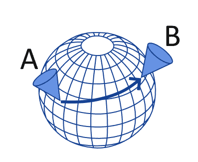
The haversine formula is frequently used for this purpose, as it gives us a way to relate latitudes and longitudes to great circle distances.

2.2. What Are Great Circle Distances?

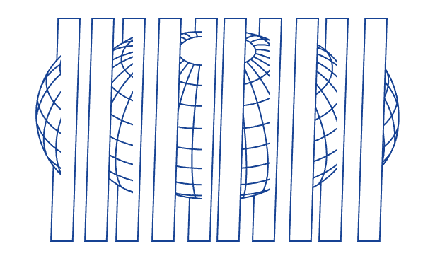
The most important concept for the haversine formula is that of a great circle in a sphere. We can think of the great circles as the intersections between some particular planes and a spherical surface. A sphere, whose surface is spherical, can be intersected by a plane in an infinite number of ways:

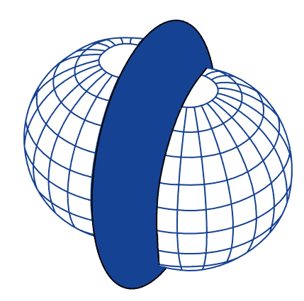
Of these planes, only a subset, however, also intersects the center of the sphere. If a plane intersects the center of the sphere, we call a great circle the collection of points that comprise the intersection with that sphere’s surface:

When we have two points on a spherical surface, we can measure their distance as the length of the path that joins them in the only great circle that goes through them. This path is also called the geodesic that connects the two points, and it’s the shortest path that’s bound to the spherical surface itself.

2.3. But Isn’t the Earth Flat?

If we’re moving in a three-dimensional flat space, we don’t need to consider great circles when calculating distances. We can, in fact, simply measure the length of the direct line connecting the two points and consider that as the shortest distance required to reach one from the other:

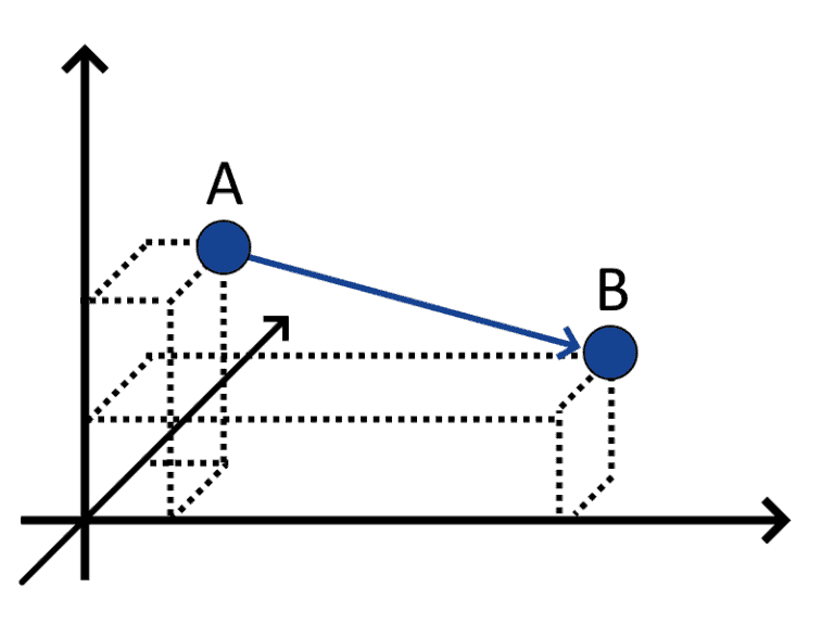
This type of distance is called Euclidean distance, and it’s appropriate for flat surfaces. The fact that Euclidean distances well approximate real-world distances on Earth for short scales is, of course, a good argument in favor of the idea that Earth is mostly flat. If, however, we consider larger scales, our job might become more complex and our Euclidean approximation less good as the distance between points increases.

2.4. Not Only for Earth’s Surface

There are, however, other situations, in addition to the travel across Earth’s surface, when we may have to use great circle distances.

We may, for example, be restricted to travel along paths with constant gravitational potential, as is the case when orbiting a body. This is the case if we’re in a geostationary orbit around Earth, and therefore we’re bound to a surface of uniform gravitational potential:

Another similar situation may arise if we conduct flight planning for airline routes. The route for an aircraft includes the altitude that an airplane has to maintain during a section of the travel path. When the altitude is constant, we can say that the movement takes place on a great circle around Earth:

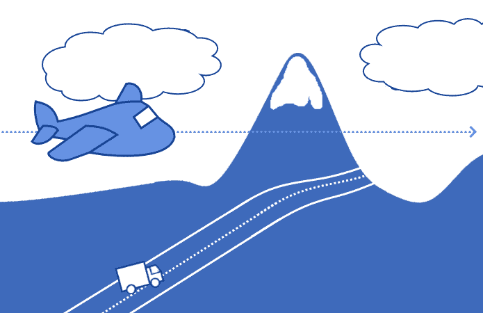
That circle isn’t located on the surface of the Earth but rather on a spherical surface that has the same center and larger radius as Earth’s.

In practice, though, great circles often relate to maintaining the same distance from the center of the Earth and therefore have something to do with gravity. However, even if we’re not bound by gravitational constraints, we might still be traveling along a great circle for other reasons.

Consider, for example, the motion of electrons around an atom:

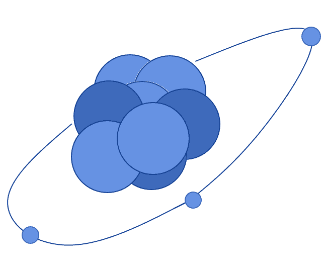
The force that generates the curved motion is electromagnetic, not gravitational, and yet the resulting motion takes place along a great circle around the nucleus. In general, if the motion we’re studying relates to movement across a spherical surface, then we can apply the haversine formula to calculate its length.

2.5. What Should a Distance Formula Contain?

We can now draft some expectations about the content of a formula for calculating distances over great circles in a spherical surface.

We know that the radius of the sphere somehow matters, and therefore that the greater the radius of a sphere, the larger the distance to travel between any two points of its surface.

This, therefore, tells us that the distance should be a monotonically increasing function of the radius of the sphere. If $r$ is the radius and $d(r)$ is the distance as a function of $r$ , we can thus say that $r_1 > r_2 \to d(r_1) > d(r_2)$ .

We can also imagine measuring the degenerate distance between two points that correspond to one another, $A \equiv B$ . By definition the distance $d_{AB}(r)$ is expected to be zero, for any value assumed by $r$ . There is, therefore, an operator $\textbf{h(A,B)}$ which equals zero when the two points $\textbf{A}$ and $\textbf{B}$ correspond, and which multiplies the radius $r$ in the formula for $d_{AB} = d(r, h(A,B))$ , such that $h(A,B) = 0 \to d(r, h(A,B)) = 0\ \forall r \in \mathbb{R}^+$ .

The operator $h(A,B)$ is thus lower-bound by 0. Further, because the distance between two points on a spherical surface is maximum if the two points are opposite with respect to the center, the operator $\textbf{h(A, B)}$ is also upper bound. Because we know that $r$ multiplies $h(A,B)$ in $d$ ‘s formula, and because the distance $d$ is upper bound by $r \pi$ , this means that $h(A,B) = \pi$ if $A$ and $B$ are opposite.

This is therefore the list of constraints to a great circle distance formula that we discussed so far:

$d_{AB} = r \times h(A, B)$
$r = 0 \to d_{AB} = 0 \rightarrow A \equiv B$
$r_1 > r_2 \to d_{AB}(r_1) > d_{AB}(r_2)$
$A \equiv B \leftrightarrow h(A,B) = 0$
$0 \leq h(A,B) \leq \pi$
$0 \leq d_{AB} \leq r \pi$

The haversine formula satisfies all of these requirements. In the next section, we’ll see how to derive it from considerations regarding distances in flat spaces and then from the application of trigonometric laws to curved spaces.

3. Distances on Flat and Spherical Surfaces

3.1. Euclidean Distance

In flat surfaces, we normally calculate distances between points by using the $L^2$ norm of the vectors that represent the two points. The $L^2$ norm is what we earlier called the Euclidean distance.

In bidimensional surfaces, if $A = (x_a, y_a)$ and $B = (x_b, y_b)$ are two points, we can use Pythagora’s equivalence to calculate the distance $d(A,B)$ as $d(A,B) = \sqrt{(B_x - A_x)^2 + (B_y - A_y)^2}$ :

More in general, if the vector space is $n$ -dimensional, we can calculate distances as $d(A,B) = \sqrt{\sum_{i=1}^n (B_i - A_i)^2}$ , where $A_i$ is the $i$ -th component of $A$ .

3.2. Distance by Cosine

If, however, the bidimensional plane is polar, one of the two components of the point-vector no longer indicates distances; but rather, an angle:

For this reason, the previous formula doesn’t apply to polar coordinate systems. If we define the points $A = (r_A, \theta_A)$ and $B = (r_B, \theta_B)$ , we can then compute their distance as $d(A,B) = \sqrt{r_A^2 + r_B^2 - 2 r_A r_B \cos (\theta_A - \theta_B)}$ .

For a surface with positive curvature, however, this is inapplicable. The considerations we made so far are, in fact, valid only for distances calculated on planar surfaces but are not generally valid otherwise.

For this reason, we will now see how to extend the polar coordinate system to the three dimensions first, and then how to calculate distances in the new system.

4. Haversine Formula

4.1. Three-Dimensional Polar Coordinate Systems

There are two main methods for extending a polar coordinate system to the third dimension.

The first is to consider the additional, third dimension, as the distance from an arbitrarily selected plane, orthogonal to the axis of the planar polar system:

This system is called a cylindric coordinate system. The other option, which is the one that we use in geospatial analysis, takes instead the name of a spherical coordinate system.

A spherical coordinate system is a polar system in which the extra dimension is also polar. In it, a spherical surface is defined as the set of points with the constant radial distance from the origin:

In a spherical coordinate system, we can also define great circles as the set of points located at the intersection between a plane passing through the origin, and the spherical surface itself, as we did earlier:

In spherical coordinate systems, distances between two points on a spherical surface are normally defined as great circle distances. This means that we measure it as the length of the arc of the great circle that comprises the two points. Since only one great circle passes through any given pair of points on a spherical surface, this distance is unique.

4.2. Definition of the Haversine Formula

We can now define the formula of haversine for calculating the distance between two points in the spherical coordinate system. The formula itself is simple, and it works for any pair of points that are defined according to their radial coordinates for a given radius:

Let’s define the two points $A$ and $B$ according to their respective latitudes $\phi$ and longitude $\lambda$ , as $A = (\phi_A, \lambda_A)$ and $B = (\phi_B, \lambda_B)$ , respectively, expressed in radians. Let’s also define the great circle distance between $A$ and $B$ as $d_{AB}$ .

Since $d_{AB}$ is an arc of a great circle with radius $r$ and central angle $\Theta$ , we know that $d_{AB} = r \times \Theta$ . In this system, the law of haversine $\text{hav}(\Theta)$ corresponding to the central angle $\Theta$ is:

$\text{hav}(\Theta) = \text{hav}(\phi_B - \phi_A) + \cos(\phi_B) \cos(\phi_A) \text{hav}(\lambda_B - \lambda_A)$

Once we compute $\text{hav}(\Theta)$ for the pair of points $(A, B)$ , we can then calculate $d_{AB}$ by using the inverse haversine function $\Theta = \text{archav}(\text{hav}(\Theta))$ . If we do that, we can finally calculate $d_{AB}$ as:

$d_{AB} = r \times \text{archav}(\text{hav}(\Theta))$

In its computation, we then simply replace $\text{hav}(\Theta)$ with its full expression defined above, in terms of the latitudes $\phi_A, \phi_B$ and longitudes $\lambda_A, \lambda_B$ of the points $A$ and $B$ .

4.3. The Earth Isn’t Spherical Though

This equation is parametric for the radius $r$ of the spherical surface. In the case of coordinates on Earth’s surface, which isn’t perfectly spherical, it’s common to use an approximate measure for the radius. This is because the radius of the surface varies between $\min(r) \approx 6356 \text{km}$ and $\max(r) \approx 6378 \text{km}$ , so an average value is needed.

In general, the value of $\overline{r} = 6371 \text{km}$ is the most commonly used. However, if we have prior knowledge that the two points are placed closer to the poles or the equator, we might then consider replacing it with $\min(r)$ or $\max(r)$ , respectively.

5. Conclusion

In this article, we studied the haversine formula for calculating great circle distances in spherical surfaces.

We first studied the rationale behind the formula by identifying examples of motions that take place along great circles.

Then, we discussed the problem of calculating distances in the Cartesian and polar coordinate system.

Finally, we generalized the problem of calculating distances to polar spherical systems. In that context, we then studied the haversine formula for great circle distances on spherical surfaces.

Full Archive

About Baeldung

Core Concepts

Operating Systems

Artificial Intelligence

Graph Theory

Latex