Graph Auto-Layout Algorithm | Baeldung on Computer Science

1. Overview

In this tutorial, we’ll study various techniques for designing the layout of graphs.

We’ll first start by discussing the different principles of convenience and aesthetics that should orient us when drawing graphs. Then, we’ll see some possible layouts for alternative representations of them.

Lastly, we’ll also study two algorithms for the automatic layout of a graph in a plane.

At the end of this tutorial, we’ll be familiar with the criteria for designing the layout of graphs, and we’ll know how to automatically draw them.

2. Representation of Graphs on a Plane

2.1. Representation, Human Perception, and Meaning

The problem of representation of graphs relates to the idea that images, in human perception, have to be interpreted in order to produce understanding. The images themselves are abstract representations over real-world objects, which allow an observer to evoke those objects into their minds:

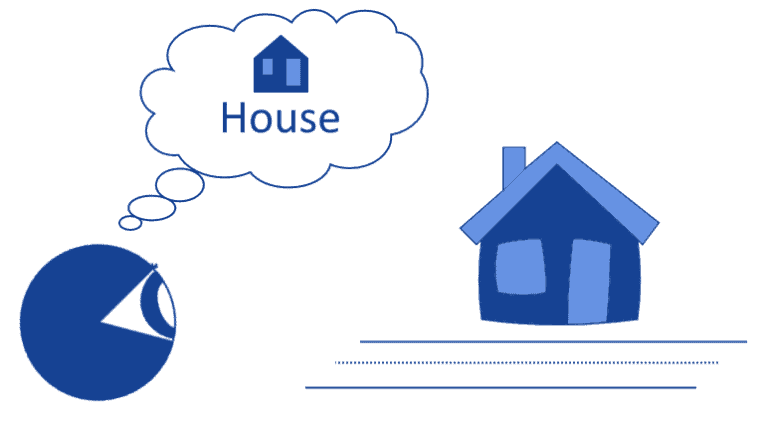
Due to their intrinsic variability, however, different images that represent the same real-world objects can evoke different mental objects into the reader’s mind. If we frame an image as a map $f$ to a real-world object, such that $f: \text{image} \mapsto \text{object}$ , we can therefore say that this map $f$ is surjective because multiple images can map to the same reality.

This is what is meant with the old adagio that says “the map isn’t the territory”. If we want to extend this consideration to graphs, we can do so by using a formula such as “the image isn’t the graph isn’t the territory”.

We know that we can represent a graph $G(V, E)$ as a set of vertices $V$ and a set of edges $E$ . We also know that multiple formal representations of them exist, such as edge lists, adjacency matrices, and adjacency lists. For this introductory section, we’ll be using a sample directed graph $G(\{1, 2, 3, 4, 5, 6\}, E)$ , with the following adjacency list:

The edge list won’t change unless otherwise specified. We’ll shortly see how we can represent the same graph in a variety of different ways, and what are the consequences for the interpretation that we assign to it.

2.2. But It’s Just a Graph!

We can also disagree with the conceptual framework we just presented, though. We can, in fact, naively claim that any arbitrary representation of a graph would be as informative as any other representation of the same graph.

This is a theory called naive realism for the human perceptual system. The theory states that no matter the object of perception, the human immediately understands it without any preliminary processing or aprioristic bias:

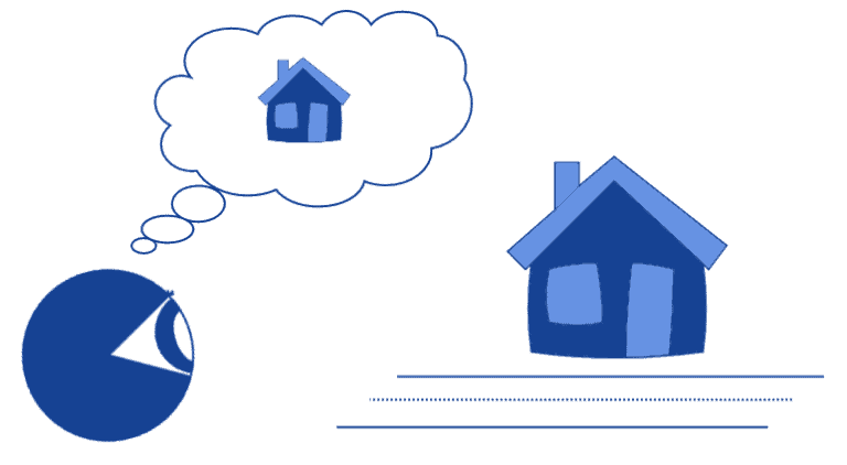
The theory also implies that, subsequently, any two humans would obtain the same understanding upon perceiving the same object:

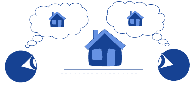
This theory has however been already falsified through theoretical reasoning and, empirically, also in relation to graphs and charts. This also means that when we draw graphs on a plane, it actually matters the technique that we use, and different methods produce different understandings with our readers.

3. Geometrical Constraints

3.1. What Are These Constraints?

The representation of a graph is, first of all, limited by the geometrical constraints that we decide to impose on it. This is simply because, if we didn’t select any kind of constraints, an infinite number of possible representations exist, with each of them corresponding to some particular combinations of edge and node positions. Instead, if we apply some kind of limitation, we can then opt for one of the possible representations that best enhance the graph given its constraints.

Multiple types of constraints exist. Some of them relate to the minimization of the horizontal or vertical space occupied by the graph. Some others, to the minimization of the total surface area.

The most interesting ones, though, relate to limitations on the placement or shaping of edges. We can thus study what classes of geometrical constraints on edges exist, with respect to the sample graph that we indicated in the previous section.

3.2. Planar Straight-Line Graphs

Hereafter, we only discuss planar graphs because constraints are more intuitive to understand for them. These are graphs whose vertex and edges all lie in the same bidimensional plane, and their edges don’t intercept with one another.

The first limitation that we impose is that all edges constitute straight segments between the vertices:

This type of representation takes the name of planar straight-line drawing. This type of graph simplifies the identification of cycles between vertices since they end up placed in the same area of the drawing surface.

3.3. Orthogonal Graphs

We can also impose the constraint that all lines, edges, or parts thereof, have to be orthogonal or parallel to any other:

This representation takes the name of orthogonal drawing. Orthogonal graphs highlight the degrees of each vertex because it’s very simple to count the number of incident edges to them. Their primary limitation is that, if at least one vertex has a degree $\delta(v) > 4$ , then the graph can’t be represented as orthogonal.

3.4. Orthogonal and Straight-Line

We can also draw a graph that, simultaneously, complies with orthogonality and has edges that are straight lines. Because the particular graph we’re using doesn’t allow this representation, we’ll drop two edges from the first node this time:

This graph takes the name of the planar orthogonal straight-line graph. This technique emphasizes the importance of graph faces, which correspond to the finite surfaces that are bound by the graph’s edges, including the infinite one that surrounds them.

3.5. Upward Flow Graphs

We can also represent the graph in a way that highlights the directional flow between its vertices:

Given the upward direction of the flow of the edges, the graph takes the name of an upward planar graph. They’re also sometimes called hierarchical networks in the literature because they’re often used to represent hierarchies in organizations. This is a misnomer, however, because hierarchical networks are those that have scale-free properties, while upward graphs don’t necessarily have any.

3.6. Constraints in Non-Planar Graphs

The ones that we’ve seen here are the primary geometrical constraints that we use to orient our decision as to what graph structures to follow. Note that the decision to employ planar graphs for these examples is for merely explicative purposes, and non-planar graphs can share the same type of constraints. In that case, though, the graph will need to be represented in a hypersurface, as opposed to a bidimensional plane.

Interestingly, orthogonal straight-line graphs in 3D space allow a maximum number of incident edges to any given vertex equal to 6. This means that, if a graph has more than four but less then seven maximum incident edges in any vertex, we can consider representing it as a 3D orthogonal straight-line graph.

4. Aesthetic Criteria for Graph Representations

4.1. What Is Aesthetics?

We also need some criteria according to which we decide what specific configuration to use, given particular constraints. These criteria take the name of aesthetic because they relate to the idea that graph representations shouldn’t be simply veridical, but should also appeal to the sense of beauty in the eyes of the perceiver.

The aesthetic criteria, together with the geometrical constraints that we discussed above, then make us decide upon a particular representation rather than another.

4.2. Minimization of Edge Crossings

The first aesthetic criterion is the minimization of the number of crossings between edges. This criterion suggests that, if multiple representations for the same graph are possible, we should choose the one with the least intersections, for ease of readability:

In this case, the representation to the right is the one we prefer.

4.3. Minimization of Graph Area

The second criterion is the minimization of the area occupied by the graph. There’s some flexibility with regards to the application of this criterion because there’s a necessary tradeoff between the readability of a graph and compactness of its surface area.

Let’s look at this example:

These graphs are equivalent. The one on the right unnecessarily occupies a surface too large, while the one on the center might be difficult to read, especially if our readers have vision pathologies. The graph on the left, instead, is a good middle-way between area minimization and ease of reading.

4.4. Minimization of Bends

The third criterion relates to the minimization of bends in edges for orthogonal graphs. Bends can, in principle, be increased to any arbitrary number:

This criterion, however, suggests to keep them instead to the bare minimum that’s required to draw the graph:

4.5. Maximization of the Smallest Angle

The next criterion indicates that the smallest angle located between any two edges of the graph should be as large as possible. Let’s study this graph of order 4:

In this case, the smallest angle is the angle $\theta$ , comprised between the two edges $(1, 2)$ and $(1, 4)$ or, equivalently, between $(3,4)$ and $(1,4)$ . This angle can be extended by repositioning the vertices appropriately:

Because $\theta_2 > \theta_1$ , this makes the second representation preferable in relation to this aesthetic criterion.

4.6. Maximization of the Shown Symmetries

The last criterion consists of the displaying of the maximum number of symmetries that are present in a graph. Let’s take a look at this example:

This picture respects the aesthetic criteria of the minimization of edge crossings because it shows no overlappings between them. It also displays three axes of symmetry, which are the medians of the equilateral triangle in which the graph is embedded.

We can, however, increase the axes of symmetry to four if we rearrange the vertices in the shape of a square:

According to this last criterion, the second drawing should be preferable to the first. Notice how it’s not always possible to respect multiple criteria simultaneously, as exemplified in this paragraph. As a consequence, whenever multiple aesthetic criteria matter in the representation of a graph, we may be called upon choosing between using only some of them.

5. Algorithms for Automatic Layout

Now that we studied geometric constraints and aesthetic criteria, we can find algorithms that automate the placement of nodes on a plane, given those constraints and those criteria that we identify. These algorithms fall loosely under these categories:

Tree drawing algorithms
Force-based algorithms
Bend minimization algorithms
Dominance drawing algorithms

Here, we study the first three of these classes of algorithms.

5.1. Recursive Algorithm for Binary Trees

If the graph we’re drawing is a binary tree, we can use a recursive algorithm for placing its nodes across horizontal layers:

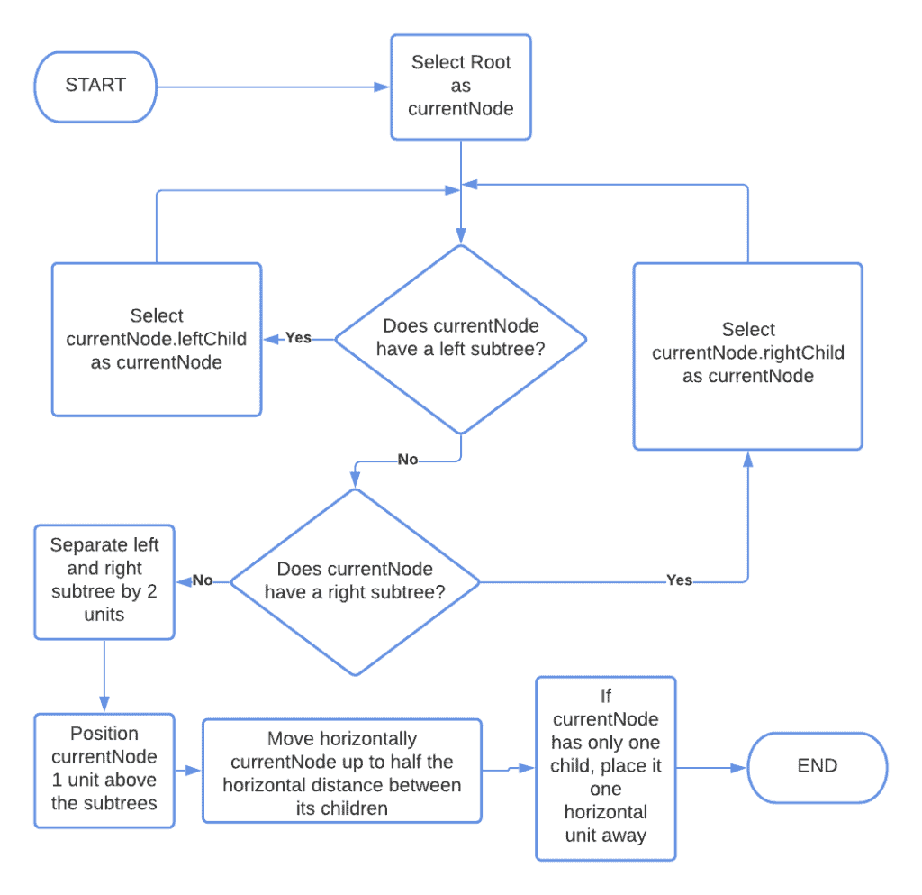
This is an example of a tree produced by that algorithm:

5.2. Force-Based Algorithms

For general classes of graphs, we can instead use force-based techniques. These are built upon the idea that edges in a graph act as springs that can pull the vertices around. Then, the graph representation is the one that minimizes the available potential energy.

In physics, a spring is an elastic material that possesses an equilibrium length and, when compressed or extended, exerts a force proportional to its deformation. In graph theory, we can imagine that the edges are springs with an equilibrium length of zero, and which then exert a force proportional to their length:

$F = -k \cdot x$

We can, therefore, imagine that each vertex is subject to a series of forces that depend on the length of its edges. Then, the vertices move in the direction that results from the combination of these forces. If we constrain the position of some vertices, we can then run the system as a dynamical simulation.

In this case, for example, we fix the vertices 2 and 3 and move vertex 1:

5.3. Bend Minimization and Network Flow

Another algorithm that we can use to change the layout of any graph into an orthogonal graph is the so-called bend minimization algorithm. We first start with any planar graph:

Then, we convert it to its high visibility form, which consists in the transformation of the vertices into parallel horizontal lines:

We then place each vertex anywhere on the corresponding line, and replace the excess line with bent edges:

Finally, we can stretch the bends and thus minimize them:

If we constrain the position of the vertices to integer coordinates in a Cartesian plane, this algorithm can be computed in $O(n^k)$ time.

6. Conclusion

In this article, we studied the principles behind the layout of graphs in drawings.

Full Archive

About Baeldung

Core Concepts

Operating Systems

Artificial Intelligence

Graph Theory

Latex