Differences Between Gradient, Stochastic and Mini Batch Gradient Descent

1. Introduction

In this tutorial, we’ll talk about Gradient Descent (GD) and the different approaches that it includes. Gradient Descent is a widely used high-level machine learning algorithm that is used to find a global minimum of a given function in order to fit the training data as efficiently as possible. There are mainly three different types of gradient descent, Stochastic Gradient Descent (SGD), Gradient Descent, and Mini Batch Gradient Descent.

2. Gradient Descent

Gradient Descent is a widely used iterative optimization algorithm that is used to find the minimum of any differentiable function. Each step that is taken improves the solution by proceeding to the negative of the gradient of the function to be minimized at the current point. In each iteration, the empirical cost $E$ of a function is calculated and the parameters used to reach the global minimum are updated accordingly. In order to find the optimal solution, this method takes into consideration the complete training dataset through every iteration, which may become time-consuming and computationally expensive.

A common problem, in the way of finding the global minima, is that GD may converge to a local minimum and may not be able to get away from it; thus, failing to approach the minimum of a function.

We can see how Gradient Descent works in the case of a one-dimensional variable in the image below:

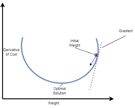
Gradient Descent technique to find global minimum

The formula of Gradient Descent that updates the weight parameter $w$ is:

$w_{i+1} = w_{i} - a\cdot \nabla_{w_{i}}J(w_{i})$

where $w$ denotes the weights that need to be updated, alpha is the Learning Rate of the algorithm, a hyperparameter that controls how much to change the model in response to the estimated error, $J$ is the cost function, while $i$ refers to the iteration index.

3. Stochastic Gradient Descent

Stochastic Gradient Descent is a drastic simplification of GD which overcomes some of its difficulties. Each iteration of SGD computes the gradient on the basis of one randomly chosen partition of the dataset which was shuffled, instead of using the whole part of the observations. This modification of GD can reduce the computational time significantly. Nevertheless, this approach may lead to noisier results than the GD, because it iterates one observation at a time.

The formula of Stochastic Gradient Descent that updates the weight parameter $w$ is:

$w_{i+1} = w_{i} - a\cdot \nabla_{w_{i}}J(x^{i}, y^{i}; w_{i})$

The notations are the same with Gradient Descent while $y$ is the target and $x$ denotes a single observation in this case.

4. Mini Batch Gradient Descent

Mini Batch Gradient Descent is considered to be the cross-over between GD and SGD. In this approach instead of iterating through the entire dataset or one observation, we split the dataset into small subsets (batches) and compute the gradients for each batch.

The formula of Mini Batch Gradient Descent that updates the weights $w$ is:

$w_{i+1} = w_{i} - a\cdot \nabla_{w_{i}}J(x^{i:i+b}, y^{i:i+b}; w_{i})$

The notations are the same with Stochastic Gradient Descent where $b$ is a hyperparameter that denotes the size of a single batch.

5. A Mathematical Approach

For a more algorithmic representation, let’s assume the scenario below:

A Hypothesis: $h_\omega(x) = \omega_0 + \omega_1 x$
Parameters that need to be updated: $\omega_0, \omega_1$
Cost Function: $J(\omega_0, \omega_1) = \frac{1}{2m} \sum^{m}_{i=1} (h_{\omega}(x^{(i)}) - y^{(i)})^2$
Aim: Minimization of $J(\omega_0, \omega_1)$ with respect to $\omega_0, \omega_1$

In the above hypothesis, the computation of $\omega$ differs for every approach. The three different methods calculate $\omega$ until it converges accordingly.

5.1. Pseudocode for Gradient Descent

$m$ is the number of training samples. We can see that, depending on the dataset, Gradient Descent may have to iterate through many samples, which can lead to being unproductive.

5.2. Pseudocode for Stochastic Gradient Descent

As we can see, in this case, the gradients are calculated on one random shuffled part out of $n$ partitions.

5.3. Pseudocode for Mini Batch Gradient Descent

Let’s assume $b$ batches.

In this case, the gradients are calculated with subsets of all observations in each iteration. This algorithm converges faster and concludes in more precise results.

6. Where Are They Used?

In machine learning and neural networks, the Gradient Descent approaches are used in backward propagation to find the parameters of the model during the training phase. Gradient Descent can be thought of as a barometer, measuring the model’s accuracy during each iteration, until the function reaches a minimum or is close/equal to zero. When a machine learning model’s accuracy is optimized via Gradient Descent it can become a powerful tool that can recognize and/or predict certain types of patterns.

7. Comparison of Gradient and Stochastic Gradient Descent

It is important to make a head-to-head comparison between the two main approaches, by analyzing the advantages and disadvantages of each one.

Gradient Descent:

Stochastic Gradient Descent:

Mini Batch Gradient Descent is the bridge between the two approaches above. By taking a subset of data we result in fewer iterations than SGD, and the computational burden is also reduced compared to GD. This middle technique is usually more preferred and used in machine learning applications.

8. Conclusion

In this article, we walked through Stochastic Gradient Descent techniques. In particular, we discussed how these different algorithms work and their approach to reaching the global minimum of a function. Finally, we talked in detail and analyzed the advantages and disadvantages of each method, and we found why the most commonly used algorithm is the Mini Batch Gradient Descent.

Full Archive

About Baeldung

Core Concepts

Operating Systems

Artificial Intelligence

Graph Theory

Latex