Introduction to Gibbs Sampling | Baeldung on Computer Science

1. Intro

In this article, we’ll describe one sampling technique called Gibbs sampling. In statistics, sampling is a technique for selecting a subset of individuals from a statistical population to estimate the characteristics of the whole population. By sampling, it’s possible to speed up data collection to provide insights in cases where it’s infeasible to measure the whole population.

One sampling technique for obtaining samples from a particular multivariate probability distribution is Gibbs sampling.

2. What Is Sampling?

As we mentioned above, sampling is a way of selecting a subset of elements from a given population. By using a proper way of sampling, we can select a smaller subset representing the whole population.

After that, we can work with that subset, and all conclusions that apply to the subset will also apply to the whole population.

Some of the sampling methods are:

Random sampling
Interval sampling
Stratified sampling
Cluster sampling

There are many different applications of sampling. Basically, in every task where we need to derive an approximation with a subset of data, we need to do some kind of sampling.

For example, while surveying our city, we need to sample a group of people that will represent the whole population. In machine learning, when we need to split the data into training and validation sets, one way of doing so is stratified cross-validation which refers to stratified sampling.

In a factory, a food technologist can sample several products and, based on their quality, determine the quality of the whole product stock and others.

3. Gibbs Sampling

Gibbs sampling is a way of sampling from a probability distribution of two or more dimensions or multivariate distribution. It’s a method of Markov Chain Monte Carlo which means that it is a type of dependent sampling algorithm. Because of that, if we need independent samples, some samples from the beginning are usually discarded because they may not accurately represent the desired distribution.

The main point of Gibbs sampling is that given a multivariate distribution, it’s simpler to sample from a conditional distribution than from a joint distribution. For instance, instead of sampling directly from a joint distribution $P(x, y)$ , Gibbs sampling propose sampling from two conditional distribution $P(x| y)$ and $P(y| x)$ .

For a joint distribution $P(x, y)$ , we start with a random sample $(x^{(0)}, y^{(0)})$ . Then we sample $x^{(1)}$ from the conditional distribution $P(x| y^{(0)})$ and $y^{(1)}$ from the conditional distribution $P(y| x^{(1)})$ . Analogously, we sample $x^{(k)}$ from $P(x| y^{(k-1)})$ and $y^{(k)}$ from $P(y| x^{(k)})$ .

4. Gibbs Sampling Definition

Suppose we want to obtain $n$ samples of $\strong{X} = (x_{1}, x_{2}, .., x_{d})$ from a joint distribution $P(x_{1}, x_{2}, .., x_{d})$ . Lets denote the $i$ -th sample as $\strong{X}^{(i)} = (x_{1}^{(i)}, x_{2}^{(i)}, .., x_{d}^{(i)})$ . The algorithm for Gibbs sampling is:

5. Example of Gibbs Sampling

To better explain this method, we will present a simple example. Let’s assume that we have two events $A$ and $B$ . Assume that the joint probability that the event will happen is given as:

$P(A\, and\, B) = 0.2$ (both events will happen)
$P(A\, and\, not\, B)$ = 0.4 (only event A will happen)
$P(not\, A\, and\, B)$ = 0.3 (only event B will happen)
$P(not\, A\, and\, not\, B)$ = 0.1 (neither A nor B will happen)

Suppose that we want to sample from the joint distribution above. We need to generate a sequence of pairs $(x, y)$ where $x, y \in \{0, 1\}$ . For example, $(1, 0)$ indicates that only event A has happened.

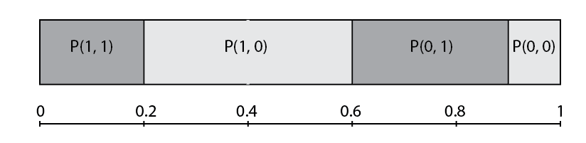
Of course, there is a simple way of sampling from the joint distribution above by taking a unit interval and dividing it into four parts, where the area of each part is equal to the probability above.

For example, we can generate a random number $n$ between $0$ and $1$ . If $n$ is between $0$ and $0.2$ , then our sample is $(1, 1)$ , if $n$ is between $0.2$ and $0.6$ , our sample is $(1, 0)$ , and analogously for others:

For this simple example, the method with unit interval is more convenient than Gibbs sampling but for some more complicated examples, especially with continuous distributions, we can’t use this method.

5.1. Conditional Distribution in Gibbs Sampling

In the Gibbs sampling method, we need to calculate conditional distribution $P(A| B)$ and $P(B| A)$ . For example, to calculate $P(A | B=1)$ , we normalize values $P(A\, and\, B) = 0.2$ and $P(not\, A\, and\, B) = 0.3$ by their sum $0.5$ and get:

$P(A=1| B=1) = 0.4$
$P(A=0| B=1) = 0.6$

Similarly for $P(A | B=0)$ , we have:

$P(A=1| B=0) = 0.8$
$P(A=0| B=0) = 0.2$

For the $P(B| A)$ values are:

$P(B=1| A=1) = 0.333$
$P(B=0| A=1) = 0.666$
$P(B=1| A=0) = 0.75$
$P(B=0| A=0) = 0.25$

Once we know all conditional distributions, we can start with the Gibbs sampling algorithm. Assume that the initial random sample is $(x^{(0)}, y^{(0)}) = (1, 0)$ . Now we need to sample $x^{(1)}$ from the conditional distribution $P(x| y^{(0)}) = P(x| 0)$ . From the above, we have that probability for $x^{(1)} = 1$ is $0.8$ and for $x^{(1)} = 0$ is 0.2. Let’s assume that we sample $1$ or $x^{(1)} = 1$ .

Now we need to sample $y^{(1)}$ from the conditional distribution $P(y| x^{(1)}) = P(y| 1)$ . From the above, we have that probability for $y^{(1)} = 1$ is $0.333$ and for $y^{(1)} = 0$ is $0.666$ . Let’s assume that we sample $1$ or $y^{(1)} = 1$ . It means that our second sample is equal to $(1, 1)$ and our sample set is currently $S = \{(1, 0), (1, 1)\}$ .

After this, we continue to sample other elements until all elements for the set $S$ are not generated.

6. Conclusion

In this article, we explained what does represent the term sampling. Our main goal was to explain Gibbs sampling using a formal definition, simple explanation, and simple example. Gibbs sampling is very useful when the joint distribution is not known explicitly or is difficult to sample from directly. Still, the conditional distribution of each variable is known and easier to sample from.

Full Archive

About Baeldung

Core Concepts

Operating Systems

Artificial Intelligence

Graph Theory

Latex