What Is Markov Chain Monte Carlo? | Baeldung on Computer Science

1. Introduction

In this tutorial, we’re going to explore a Markov Chain Monte Carlo Algorithm (MCMC). It is a method to approximate a distribution from random samples. It specifically uses a probabilistic model called Markov chains. We concretely look at the so-called Metropolis-Hastings algorithm which is a type of MCMC.

2. What Is a Markov Chain?

A Markov chain is a description of how probable it is to transfer from one state into another. The probability of this transfer depends thereby only on the previous state. It may be noted that these transfer probabilities should be known, otherwise a Hidden Markov Model might be the correct choice. To clarify how a Markov chain works, let’s have a look at an example.

2.1. Example

We have a restaurant that changes its menu daily. The chef is a very simple man so the only food he cooks is either fish or pasta. The choice of food he cooks can be described with the following probabilities:

$P(\text{Fish}\,\vert \, \text{Fish}) = 0.2$
$P(\text{Fish} \,\vert \, \text{Pasta}) = 0.7$
$P(\text{Pasta} \,\vert \, \text{Fish}) = 0.8$
$P(\text{Pasta} \,\vert \, \text{Pasta}) = 0.3$

$\textbf{P(A} | \textbf{B)}$ signifying A is today’s food given yesterday’s food B.
For example, the probability for the chef to cook fish given the already cooked fish yesterday is 20%:

2.2. Equilibrium State

Another important term in the language of Markov chains is the equilibrium state. When we look at our Markov chain definition we might ask, how high the probability for fish will be in one week or even further in the future. To calculate this probability we transform our table into a matrix:

$T = \left[ {\begin{array}{cc} 0.2 & 0.8 \\ 0.7 & 0.3 \\ \end{array} } \right]$

Now we calculate the probability of fish in one week given the dish from the previous day. We can do this by simply multiplying the matrix by itself 7 times:

$T_{7} = \left[ {\begin{array}{cc} 0.2 & 0.8 \\ 0.7 & 0.3 \\ \end{array} } \right]^{7} = \left[ {\begin{array}{cc} 0.4625 & 0.5375 \\ 0.4703125 & 0.5296875 \\ \end{array} } \right]$

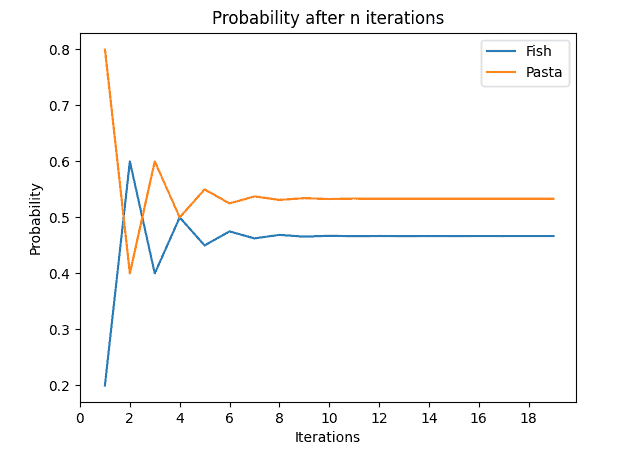
We can now ask ourselves, how will this matrix behave even further away in the future? The answer is, that this matrix will reach a so-called equilibrium state after being multiplied by itself a sufficient number of times. Thus, the matrix does not change anymore after self-multiplying it any further. In the diagram below, we can see the probabilities with the assumption of fish on the previous day:

The diagram for pasta being served on the previous day looks very similar:

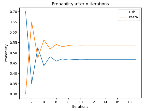
The reason for that is that it has the same equilibrium probabilities, as we can see in the equilibrium matrix:

$E = \left[ {\begin{array}{cc} 0.466 & 0.533 \\ 0.466 & 0.533 \\ \end{array} } \right]$

It can be noted, that not every Markov chain has a stationary state. We’ll later see how we can construct one that always fulfills this condition.

3. Markov Chain Monte Carlo

In the following, we’ll describe the so-called Metropolis-Hasting algorithm, which is a type of MCMC algorithm. Our goal is to find a distribution $P$ which is proportional to the distribution we draw samples from, let’s call it $f$ .

To do so, we utilize a Markov chain to model how probable it is for one of the samples given the one we drew before. We can formalize this probability as we have already seen in the explanation of Markov chains, as:

$P(x' = p' | x = p)$ , $p$ being the last sample and $p'$ being the current one. Let’s explore the algorithm in detail.

3.1. Metropolis-Hasting

Let’s go through the algorithm step by step.

As already mentioned, all we need is our sample function $f$ and a number of steps we want our algorithm to iterate, $N$ . The MCMC is constructed in a way that it always converges to the target distribution after a sufficient number of steps.

What we retrieve from the algorithm is an acceptance ratio, which tells us how close the Markov chain is to its stationary distribution and an array of states. The state describes the probability of obtaining the current sample given our last sample. Thus it is a number between 0 and 1. Later we can create a histogram from the array of states to receive our target distribution.

First of all, we generate a random number as our starting point, we call it $x$ .

Following this, we step through our loop executing the following steps each time:

we generate a new sample from our prior distribution, plugging $x$ into it
we check how probable our new sample is, given our old sample. As we can see, we use $\frac{f(x)}{f(x')}$ , meaning the scaling of our distribution we draw from does not matter. Thus resulting in $\frac{f(x)}{f(x')} = \frac{P(x)}{P(x')}$ , making it calculable without knowing the posterior
we check if this conditional probability is high enough to add the state to our Markov chain $ss$ . If it is not, we add our old state to the chain. We then use our new current state to generate a new sample. This procedure is also called Random Walk.

This algorithm allows us to stay in high probability areas because every time we change from an area of high probability to one with low probability, we get a low acceptance probability $\textbf{R}$ .

3.2. Acceptance Probability

In the center of the Metropolis-Hastings algorithm is the acceptance probability $R$ . How can we derive such a formula? And even more important is: How can we ensure that it converges towards the posterior distribution?

To go back to our Markov example from the beginning, we remind ourselves that our chain had an equilibrium state. This state is also called the stationary state. Applying this to our Markov chain from the algorithm, we note that it converges towards the target distribution as the chain converges to its stationary state.

For our markov chain to converge to a stationary it needs to fullfill the following balancing condition:

$P(x'| x)P(x) = P(x | x') P(x')$

which can be written as:

$\frac{P(x')}{P(x)} = \frac{P(x' | x)}{P(x | x')}$

Following this, we can define the so-called acceptance distribution $A(x's,x)$ . It describes the probability to accept the state $x'$ and can be formalized by

$A(x',x) = P(x',x)g(x' | x)$

It describes the probability to accept state $x'$ given $x$ . We can thus formulate:

$\frac{A(x,x')}{A(x',x)} = \frac{P(x)}{P(x') } \frac{g(x'|x)}{g(x' | x)}$

For the last step we only have to choose a criterion to accept a sample. We choose the Metropolis acceptance criterion:

$R = min(1, \frac{P(x')}{P(x)} \cdot \frac{g(x' | x)} {g(x | x ')})$

3.3. Toy Example

To see what we can do with our resulting Markov chain and to get an outlook on the applications of the Metropolis-Hastings algorithm, we take a look at an example. For this matter, we use samples from a normal distribution with a variance $\sigma^{2}$ of 3:

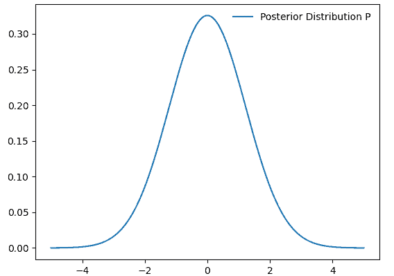
In the plot, we can see the probability density function of our posterior distribution $P$ . We do not know this distribution directly, only a numerical function $f$ which is proportional to it and from which we sample.

In the next step, we sample from this distribution and plot the histogram of the resulting Markov chain:

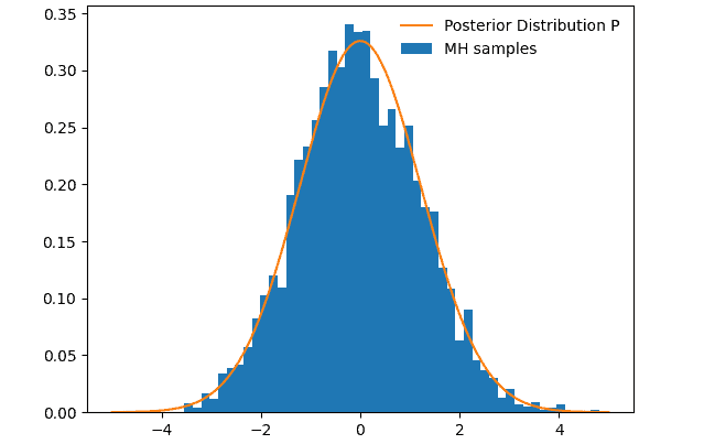
After 5000 steps we can already see how the samples start converging towards the posterior distribution $P$ .

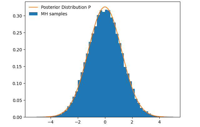
After 100 000 steps we can see how well the samples converge:

Other interesting examples include i.e. the decryption of messages and the Monte Carlo Tree Search.

4. Comparison to Other Sampling Algorithms

While we used the MCMC algorithm to sample from a 1D Distribution, its main use lies in the distribution analysis of multi-dimensional problems. Its core disadvantage in the 1D case lies in the fact that its samples are correlated. It, therefore, results in a lower sampling resolution. We can solve this by other types of sampling algorithms such as adaptive rejection sampling.

Another challenge that arrives with the MCMC algorithm is how fast our Markov chain converges towards our target distribution. This property is highly dependent on the number of parameters and the configuration of the MCMC algorithm. The Hamiltonian Monte Carlo algorithm solves this challenge by generating larger steps between the samples furthermore resulting in a smaller correlation between them.

5. Conclusion

In this article, we went through the MCMC algorithm step by step, specifically the Metropolis-Hastings variant. We have seen how we can create a Markov chain by selecting samples from our distribution. Furthermore, we proved that this chain then converges towards our posterior distribution. Following this, we looked at how to apply the algorithm in a concrete example and how to compare it to other methods.

Full Archive

About Baeldung

Core Concepts

Operating Systems

Artificial Intelligence

Graph Theory

Latex