Understanding Time Complexity Calculation for Dijkstra Algorithm

1. Introduction

Dijkstra’s algorithm is used to find the shortest path from a starting node to a target node in a weighted graph. The algorithm exists in many variations, which were originally used to find the shortest path between two given nodes. Now they’re more commonly used to find the shortest path from the source to all other nodes in the graph, producing a shortest path tree.

In this tutorial, we’ll learn the concept of Dijkstra’s algorithm to understand how it works. At the end of this tutorial, we’ll calculate the time complexity and compare the running time between different implementations.

2. The Algorithm

The algorithm, published in 1959 and named after its creator, Dutch computer scientist Edsger Dijkstra, can be applied to a weighted graph. The algorithm finds the shortest path tree from a single source node by building a set of nodes with minimum distances from the source.

2.1. Condition

It’s important to note the following points:

Dijkstra’s algorithm works only for connected graphs.
It works only for graphs that don’t contain any edges with a negative weight.
It only provides the value or cost of the shortest paths.
The algorithm works for directed and undirected graphs.

2.2. Dijkstra’s Algorithm

Dijkstra’s algorithm makes use of breadth-first search (BFS) to solve a single source problem. However, unlike the original BFS, it uses a priority queue instead of a normal first-in-first-out queue. Each item’s priority is the cost of reaching it from the source.

Before going into the algorithm, let’s briefly review some important definitions.

The graph has the following:

vertices, or nodes, denoted in the algorithm by $v$ or $u$
weighted edges that connect two nodes: ( $u$ , $v$ ) denotes an edge, and $w(u, v)$ denotes its weight

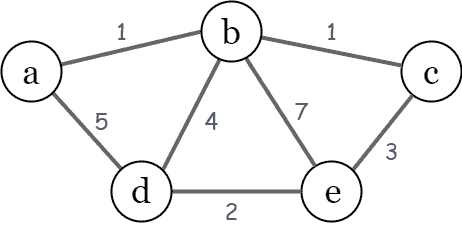
The following example illustrates an undirected graph with the weight for each edge:

To implement Dijkstra’s algorithm, we need to initialize three values:

$dist$ – an array of the minimum distances from the source node $s$ to each node in the graph. At the beginning, $dist(s) = 0$ , and for all other nodes $v$ , $dist(v) = \infty$ . The $dist$ array will be recalculated and finalized when the shortest distance to every node is found.
$Q$ – a priority queue of all nodes in the graph. At the end of the progress, $Q$ will be empty.
$S$ – a set to indicate which nodes have been visited by the algorithm. At the end of the progress, $S$ will contain all the nodes of the graph.

The algorithm proceeds as follows:

Pop the node $v$ with the smallest $dist(v)$ from $Q$ . In the first run, source node $s$ will be chosen because $dist(s) = 0$ in the initialization.
Add node $v$ to $S$ , to indicate that $v$ has been visited.
Update $dist$ values for each adjacent node of the current node $v$ as follow: (1) if $dist(v) + weight(v, u) < dist(u)$ , so update $dist(u)$ to the new minimal distance value, (2) otherwise no updates are made to the $dist(u)$ .
The progress will stop when $Q$ is empty, or in other words, when $S$ contains all nodes, which means every node has been visited.

Let’s go through an example before coding it with the pseudocodes.

2.3. Examples

Given the following undirected graph, we’ll calculate the shortest path between the source node $e$ and the other nodes in our graph. To begin, we mark $dist(c) = 0$ ; for the rest of the nodes, the value will be $\infty$ as we haven’t visited them yet:

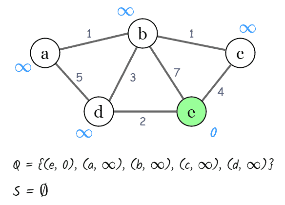
At this step, we pop a node with the minimal distance (i.e., node $e$ ) from $Q$ as the current node, and mark the node $e$ as visited (add node $e$ to $S$ ). Next, we check the neighbors of our current node ( $b$ , $c$ , and $d$ ) in no specific order.

At the node $b$ , we have $dist(b) = \infty > dist(e) + weight(e, b) = 0 + 7 = 7$ , so we update $dist(b) = 7$ . Similarly, we update $dist(c) = 4$ and $dist(d) = 2$ . In addition, we update the priority queue after recalculating the distances of these nodes:

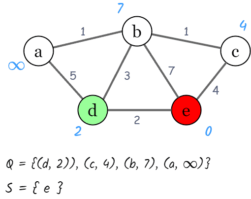
Now we need to pick a new current node by popping from the priority queue $Q$ . That node will be un-visited with the smallest minimum distance. In this case, the new current node is $d$ with $dist(d) = 2$ . Then we repeat adjacent node distance calculations.

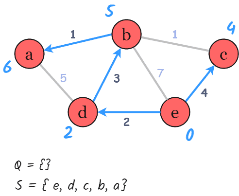
After repeating these steps until $Q$ is empty, we reach the final result of the shortest-path tree:

2.3. Pseudocode

The following pseudocode shows the details of Dijkstra’s algorithm:

algorithm Dijkstra(G, source):
    // INPUT
    //     G = the input graph (G = (V, E))
    //     source = the source node

    // Initialization
    for v in V
        initialize dist[v] = infinity
    
    dist[source] <- 0
    
    for v in V:
        add v to Q
    
    S <- empty set

    // The main loop for the algorithm
    while Q is not empty:
        v <- vertex in Q with min dist[v]
        remove v from Q
        add v to S

        for neighbour u of v:
            if u is in S:
                continue // if u is visited then ignore it

            alt <- dist[v] + weight(v, u)
            if alt < dist[u]:
                dist[u] <- alt // update distance of u
                update Q

    return dist

For a more in-depth explanation of Dijkstra’s algorithm using pseudocodes, we can read an Overview of Dijkstra’s Algorithm. Then we can learn how to implement Dijkstra Shortest Path Algorithm in Java.

3. Implementations and Time Complexity Analysis

There are multiple ways we can implement this algorithm. Each way utilizes different data structures to store the graph, as well as the priority queue. Thus, the differences between these implementations leads to different time complexities.

In this section, we’ll discuss the time complexity of two main cases for Dijkstra’s implementations.

3.1. Case 1

This case happens when:

The given graph $G=(V, E)$ is represented as an adjacency matrix. Here $w[u, v]$ stores the weight of edge $(u, v)$ .
The priority queue $Q$ is represented as an unordered list.

Let $|E|$ and $|V|$ be the number of edges and vertices in the graph, respectively. Then the time complexity is calculated:

Adding all $|V|$ vertices to $Q$ takes $O(|V|)$ time.
Removing the node with minimal $dist$ takes $O(|V|)$ time, and we only need $O(1)$ to recalculate $dist[u]$ and update $Q$ . Since we use an adjacency matrix here, we’ll need to loop for $|V|$ vertices to update the $dist$ array.
The time taken for each iteration of the loop is $O(|V|)$ , as one vertex is deleted from $Q$ per loop.
Thus, total time complexity becomes $O(|V|) + O(|V|) \times O(|V|) = O(|V|^2)$ .

3.2. Case 2

This case is valid when:

The given graph $G=(V, E)$ is represented as an adjacency list.
The priority queue $Q$ is represented as a binary heap or a Fibonacci heap.

First, we’ll discuss the time complexity using a binary heap. In this case, the time complexity is:

It takes $O(|V|)$ time to construct the initial priority queue of $|V|$ vertices.
With adjacency list representation, all vertices of the graph can be traversed using BFS. Therefore, iterating over all vertices’ neighbors and updating their $dist$ values over the course of a run of the algorithm takes $O(|E|)$ time.
The time taken for each iteration of the loop is $O(|V|)$ , as one vertex is removed from $Q$ per loop.
The binary heap data structure allows us to extract-min (remove the node with minimal $dist$ ) and update an element (recalculate $dist[u]$ ) in $O(log|V|)$ time.
Therefore, the time complexity becomes $O(|V|) + O(|E| \times log|V|) + O(|V| \times log|V|)$ , which is $O((|E|+|V|) \times log|V|) = O(|E| \times log|V|)$ , since $|E| \geq |V| - 1$ as $G$ is a connected graph.

For a more in-depth overview and implementation of the binary heap, we can read the article that explains Priority Queue.

Next we’ll calculate the time complexity using a Fibonacci heap. The Fibonacci heap allows us to insert a new element in $O(1)$ and extract the node with minimal $dist$ in $O(log|V)$ . Therefore, the time complexity will be:

The time taken for each iteration of the loop and extract-min is $O(|V|)$ , as one vertex is removed from $Q$ per loop.
Iterating over all vertices’ neighbors and updating their $dist$ values for a run of the algorithm takes $O(|E|)$ time. Since each priority value update takes $O(log|V|)$ time, the total of all $dist$ calculation and priority value updates takes $O(|E| \times log|V|)$ time.
So the overall time complexity becomes $O(|V| + |E| \times log|V|)$ .

4. Time Complexity Comparison

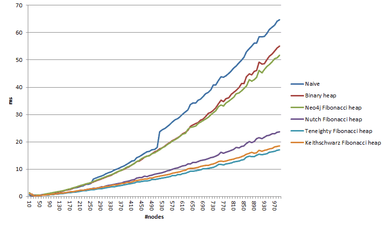
Overall, the Fibonacci heap-based implementation will run at the fastest speed. Conversely, the slowest version will be the unordered list-based priority queue version. However, if the graph is well-connected (i.e., having a huge number of edges, aka, having high density), there is not much difference between these three implementations.

For a detailed comparison of the running time with different implementations, we can read the experimenting with Dijkstra’s algorithm article.

For example, the following figure illustrates the running time comparison between six variants when the number of nodes is increasing:

5. Conclusion

In this article, we discussed Dijkstra’s algorithm, a popular shortest path algorithm on the graph.

First, we learned the definition and the process of a priority queue. Then we explored an example to better understand how the algorithm works.

Finally, we examined and compared the complexity of the algorithm in three different implementations.

Full Archive

About Baeldung

Core Concepts

Operating Systems

Artificial Intelligence

Graph Theory

Latex