Grey Wolf Optimization Algorithm | Baeldung on Computer Science

1. Intro

In this article, we’ll review the Grey Wolf Optimization (GWO) algorithm and how it works. As we can conclude from the name, this is a nature-inspired metaheuristic that is based on the behavior of a pack of wolves. Similar to other nature-inspired metaheuristics such as genetic algorithm and firefly algorithm, it explores the search space in hope of finding an optimal solution.

In summary, this is an iterative method that is used for optimization problems.

2. Inspiration

The inspiration for this algorithm is the behavior of the grey wolf, which hunts large prey in packs and relies on cooperation among individual wolves. There are two interesting aspects of this behavior:

social hierarchy
hunting mechanism

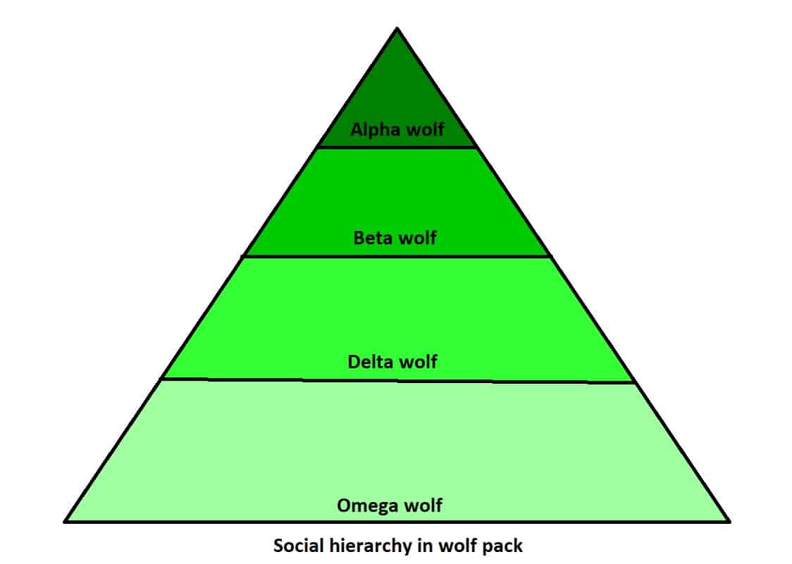
The grey wolf is a highly social animal with the result that it has a complex social hierarchy. This hierarchical system, where wolves are ranked according to strength and power, is called “dominance hierarchies”. Therefore, there are the alphas, betas, deltas, and omegas.

The alpha male and females are at the top of the hierarchy, and they lead the pack. All members of the pack have ordered within a specific rank. The wolf’s hierarchical system is not just about dominance and aggression; it also provides assistance to vulnerable members of the pack who cannot hunt for themselves.
Afterward is the beta wolf that supports the alpha wolf’s decisions and helps keep discipline within the pack.
The delta wolf is below the beta wolf in rank. They are often strong but lack leadership skills or confidence in themselves to take on leadership responsibilities.
And last, the omega wolf does not have any power at all and other wolves will quickly chase him. Omega wolf is also responsible for watching over younger wolves.

Besides social hierarchy, grey wolves have a very specific way of hunting with a unique strategy. They hunt in packs and work together in groups to separate the prey from the herd, then one or two wolves will chase after and attack the prey while the others chase off any stragglers.

Muro et al. describe the hunting strategy of the wolf pack and it includes:

approach, track and chase the prey
pursuit, harass, and encircling maneuver around the prey until it stops moving
attack the prey when it is exhausted

3. Definition

Applying the previously described methodology to our optimization problem, at each step, we’ll denote respectively the three best solutions by alpha, beta, and delta, and other solutions by omega. Basically, it means the optimization process goes with the flow of the three best solutions. Also, the prey will be the optimal solution of the optimization.

Most of the logic follows the equations:

(1) $\begin{align*} \vec{D} = |\vec{C}\cdot \vec{X}_{p}(t) - \vec{X}(t)| \end{align*}$

(2) $\begin{align*} \vec{X}(t+1) = \vec{X}_{p}(t) - \vec{A}\cdot \vec{D}, \end{align*}$

where $t$ denotes current iteration, $\vec{A}$ and $\vec{C}$ are coefficient vectors, $\vec{X}_{p}$ is the position vector of the prey and $\vec{X}$ is the position of wolf . Vectors $\vec{A}$ and $\vec{B}$ are equal to:

(3) $\begin{align*} \vec{A} = 2\vec{a}\cdot \vec{r}_{1} - \vec{a} \end{align*}$

(4) $\begin{align*} \vec{C} = 2\vec{r}_{2}, \end{align*}$

where components of $\vec{a}$ are linearly decreased from 2 to 0 through iterations and $\vec{r}_{1}$ , $\vec{r}_{2}$ are random vectors with values from $[0,1]$ , calculated for each wolf at each iteration. Vector $\vec{A}$ controls the trade-off between exploration and exploitation while $\vec{C}$ always adds some degree of randomness. This is necessary because our agents can get stuck in the local optima and most of the metaheuristics have a way of avoiding it.

Since we don’t know the real position of the optimal solution, $\vec{X}_{p}$ depends on the 3 best solutions and the formulas for updating each of the agents (wolfs) are:

(5) $\begin{align*} \vec{D}_{\alpha} = |\vec{C}_{1}\cdot \vec{X}_{\alpha} - \vec{X}|, \vec{D}_{\beta} = |\vec{C}_{2}\cdot \vec{X}_{\beta} - \vec{X}|, \vec{D}_{\delta} = |\vec{C}_{3}\cdot \vec{X}_{\delta} - \vec{X}| \end{align*}$

(6) $\begin{align*} \vec{X}_{1} = \vec{X}_{\alpha} - \vec{A}_{1}\cdot, \vec{X}_{2} = \vec{X}_{\beta} - \vec{A}_{2}\cdot, \vec{X}_{3} = \vec{X}_{\delta} - \vec{A}_{3} \end{align*}$

(7) $\begin{align*} \vec{X}(t+1) = \frac{\vec{X}_{1} + \vec{X}_{2} + \vec{X}_{3}}{3}, \end{align*}$

where $\vec{X}$ is the current position of the agent and $\vec{X}(t+1)$ is the updated one. The formula above indicates that the position of the wolf will be updated accordingly the to best three wolves from the previous iteration. Notice that it won’t be exactly equal to the average of the three best wolves but because of the vector $\vec{C}$ , it adds a small random shift. This makes sense because, from one side, we want that our agents are guided by the best individuals and from another side, we don’t want to get stuck in the local optima.

Finally, the pseudocode of GWO is:

Notice that the time complexity of the algorithm is dependent on the number of iterations, agents, and size of the vectors but generally we can approximate the time complexity as $\mathcal{O}(k\cdot n)$ , where $k$ is the number of iterations and $n$ is the number of agents.

4. Example

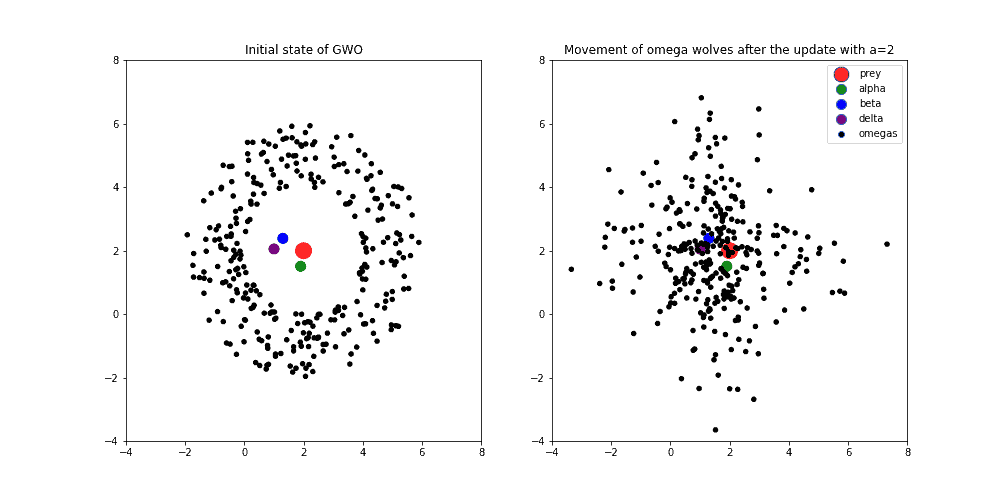
In order to better understand this algorithm, we’ll present one concrete example of the wolf pack behavior. In the image below (left), we can see the initial state of the agents, where prey or optimal solution has a red color. The closest wolves to the prey (alpha, beta, and delta) have a green, blue, and purple color respectively. Black dots represent other wolves (omegas).

Further, if we update the position of omega wolves according to the formulas explained in the previous section, we can observe the behavior of agents in the image below (right). Notice that the variable $a$ that controls the trade-off between exploration and exploitation is set to the value 2. This means that we prefer exploration overexploitation:

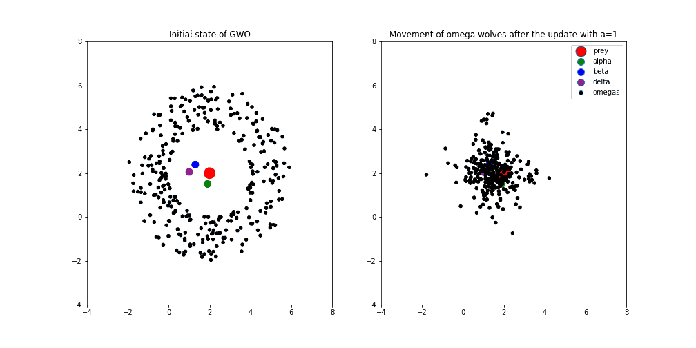
Secondly, the next image shows the behavior of the wolf pack when the variable $a$ is set to value 1. Usually, this means that we’re in the middle of the optimization process and the exploitation process increasingly appears:

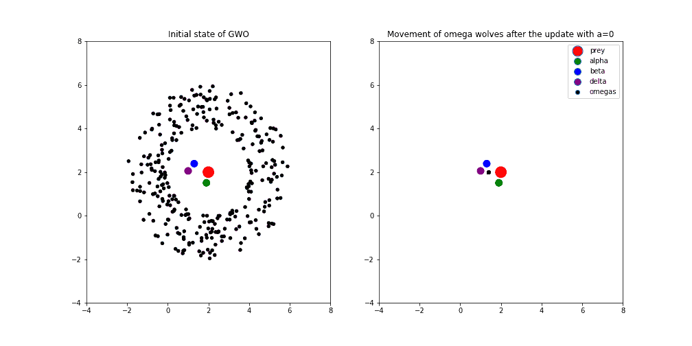
Finally, in the image below, the variable $a$ is equal to 0. It means that the optimization process is at the end and we’re hopefully converging towards the optimal solution following the best three wolves. We can see how omega wolves are gathering between the best three wolves, around the point that geometrically represents centroid between alpha, beta, and delta agents:

Notice that we didn’t update the position of alpha, beta, and delta agents just because of the comparison with the omegas. Otherwise, we update the position of all agents, and after that, we select new alpha, beta, and delta. After all, the convergence of GWO agents might look like the animation below:

5. Applications

In general, we can use this algorithm to solve a lot of different optimization problems. Below, we’ll mention only some of them that could be useful in machine learning.

5.1. Hyperparameter Tuning

One interesting application might be hyperparameter tuning of any machine learning algorithm. The main idea behind hyperparameter tuning is to find an optimum set of values for parameters in order to maximize the performance of a given algorithm.

For instance, using GWO we could optimize hyperparameters of Gradient Boosting. In that case, we can construct the position vector in a way where each of the vector components for a value has a particular hyperparameter. For example, X = (learning rate, number of trees, maximum depth). The parameters don’t have to have a numeric value at all because we can always define our own metrics for calculating the distance between agents.

5.2. Feature Selection

Another application of GWO that is also related to machine learning is feature selection. The algorithm works by constructing a set of possible features and iteratively modifying these features based on some performance measure until the desired solution is found.

This approach is a lot cheaper in terms of time complexity since the complexity for choosing the best subset of features increases exponentially with every additional variable. This is because the total number of subsets of a set with $n$ elements is $2^{n}$ . It means that if we have 30 different features as an input into the machine learning algorithm, as a result, the number of possible subsets of 30 features is $2^{30}=1.073.741.824$ !

Thus, it would be more feasible to represent 30 features as a binary vector with a size of 30 (each bit is one particular feature, 1 indicates that the feature is included and 0 that it is not). That binary vector represents the position of the agent and could be easily used by GWO or any other metaheuristics.

5.3. Other Examples

Besides the above examples, the GWO has been successfully used in solving various problems such as:

the traveling salesman problem (TSP)
the minimum spanning tree problem
non-linear equation systems
power flow problem and other

6. Conclusion

In this article, we’ve described the intuition and logic behind the GWO algorithm to provide a better understanding of how we can apply it to solve some optimization problems. We introduced this algorithm because it is quite effective, yet simple enough to be easily understood. The article explores what a GWO is, an example of how it works and provides several key considerations on the examples of applications.

Full Archive

About Baeldung

Core Concepts

Operating Systems

Artificial Intelligence

Graph Theory

Latex