Confidence Intervals | Baeldung on Computer Science

1. Introduction

In this tutorial, we’ll explain confidence intervals and how to construct them.

2. Uncertainty Quantification

Let’s introduce them with an example.

Let’s say we want to check if volleyball or basketball has a greater influence on people’s heights. The only way to be sure about the answer is to measure the heights of all professional and amateur volleyball and basketball players worldwide, but that’s impossible.

Instead, we can visit local sports clubs and measure their players’ heights. That way, we get two samples of measurements. For instance (centimeters):

$Volleyball = \begin{bmatrix}187 & 190 & 184 & 175 & 200 \\ 195 & 191 & 188 & 179 & 185 \\ 199 & 198 & 205 & 188 & 183 \\ 190 & 192 & 193 & 185 & 190 \end{bmatrix} \qquad Basketball = \begin{bmatrix}193 & 195 & 196 & 190 & 185 \\ 188 & 187 & 185 & 189 & 198 \\ 200 & 185 & 194 & 210 & 197 \\ 202 & 199 & 204 & 192 & 189 \end{bmatrix}$

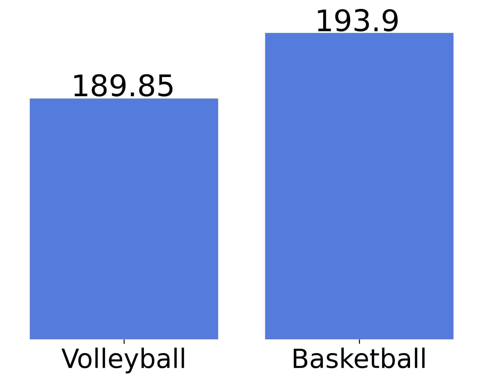
The mean heights in the sample are:

Average heights of basketball and volleyball players in a made-up sample.

Would it be justified to claim that basketball players will grow taller than those who prefer volleyball? The caveat is that we could have gotten different results had our samples been different. That’s why it isn’t sufficient to compute sample means and proportions. We also have to quantify their uncertainty.

Confidence intervals do just that: they show us the range of plausible values of a population parameter given the one we calculated using a (much smaller) sample.

3. Confidence Intervals

Let’s start with an informal definition.

3.1. Informal Definition

Let $\theta$ be the unknown value of a numeric parameter, population-wise. For instance, the average height of volleyball and basketball players or the proportion of a presidential candidate’s voters in a country’s electorate.

We can estimate $\theta$ only by analyzing samples. So, let $S=\{x_1, x_2, \ldots, x_n\}$ be a sample, and $\theta(S)$ the value calculated using $S$ .

A confidence interval for $\theta$ , given $\theta(S)$ , is a range of values $[L, U] \ni \theta(S)$ obtained through a procedure with a predefined coverage (or confidence). The confidence expresses the probability that an interval (produced by the procedure) contains the exact value of the parameter.

Let’s step back for a second. Why do we say that confidence is a characteristic of the procedure and not a specific interval?

3.2. Random vs. Specific Samples

That’s because confidence intervals are a tool of frequentist statistics. We differentiate between random and specific (or realized) samples in it.

A specific sample contains specific values; examples are the samples of volleyball and basketball players’ heights.

In contrast, a random sample comprises random variables (denoted as $X_1, X_2, \ldots, X_n$ ). Each variable in a random sample models a possible value that a specific sample can contain.

Therefore, specific samples are realizations of the corresponding random samples.

3.3. Estimators vs. Sample Statistics

When we apply the formula for $\theta$ to a random sample $\{X_1, X_2, \ldots, X_n\}$ , we get a random variable called an estimator. Let’s denote it with $\widehat{\theta}$ . For the average value, $\widehat{\theta}$ is:

$\frac{1}{n}\sum_{i=1}^{n} X_i$

In contrast, applying the formula for $\theta$ to a realized sample $\{x_1, x_2, \ldots, x_n\}$ results in a specific sample value we’ll denote as $\theta^*$ . In our example with heights, the means 189.95 and 193.9 are sample values (means), i.e., realizations of the estimator.

3.4. Formal Definition

Now, we’re ready for the formal definition.

A confidence interval with the confidence level of $100\gamma\%$ , where $\gamma \in (0, 1)$ , for the parameter whose true value is $\theta$ , estimator is $\widehat{\theta}$ , and the sample value is $\theta^*$ , is a range of values $[L, U]$ such that:

$\Pr\left\{ L \leq \theta \leq U \right\} \geq \gamma$

where:

$L$ and $U$ depend on $\theta^*$ and the distribution of $\widehat{\theta}$
The probability is calculated using the distribution of $\widehat{\theta}$

So, if we apply the procedure outputting 95% CIs to many different samples, approximately 95% will contain the actual value of the parameter of interest.

Since the probability is in the equation only through the random sample, we can ascribe the confidence level $\gamma$ to the procedure outputting the intervals and not to any specific interval it produces.

3.5. Example

In our example, $\widehat{\theta}$ is the mean of $n$ independent and identically distributed random variables. Its standardized form:

$\frac{\widehat{\theta}-\theta}{s_n/\sqrt{n}}$

where $s_n$ is the sample standard deviation (also an estimator), follows the Student’s t distribution with $n-1$ degrees of freedom. Let $t$ be its $\frac{1-\gamma}{2}$ quantile, i.e.:

$\Pr \left\{ \frac{\widehat{\theta}-\theta}{s_n/\sqrt{n}} > t\right\} = \frac{1-\gamma}{2}$

Since the Student’s distribution is symmetric, we also have:

$\Pr \left\{ \frac{\widehat{\theta}-\theta}{s_n/\sqrt{n}} < -t \right\} = \frac{1-\gamma}{2}$

So, the probability for $\frac{\widehat{\theta}-\theta}{s_n/\sqrt{n}}$ to fall between $-t$ and $t$ is $1-\frac{1-\gamma}{2}-\frac{1-\gamma}{2}=1-(1-\gamma)=\gamma$ :

$\Pr \left\{ -t < \frac{\widehat{\theta}-\theta}{s_n/\sqrt{n}} < t \right\} = \gamma$

Manipulating the expression between the curly braces, we get:

$\Pr \left\{ \widehat{\theta} - \frac{t s_n}{\sqrt{n}} < \theta <\widehat{\theta} + \frac{t s_n}{\sqrt{n}} \right\} = \gamma$

That’s our $100\gamma\%$ confidence interval.

4. Inference

We’ll focus on two cases: comparing the parameters of two populations and comparing one population’s parameter to a predefined value.

4.1. Comparing Two Populations

When we compute the 99% confidence intervals for our height means, we get $(175.05, 204.65)$ for volleyball and $(179.93, 207.97)$ for basketball:

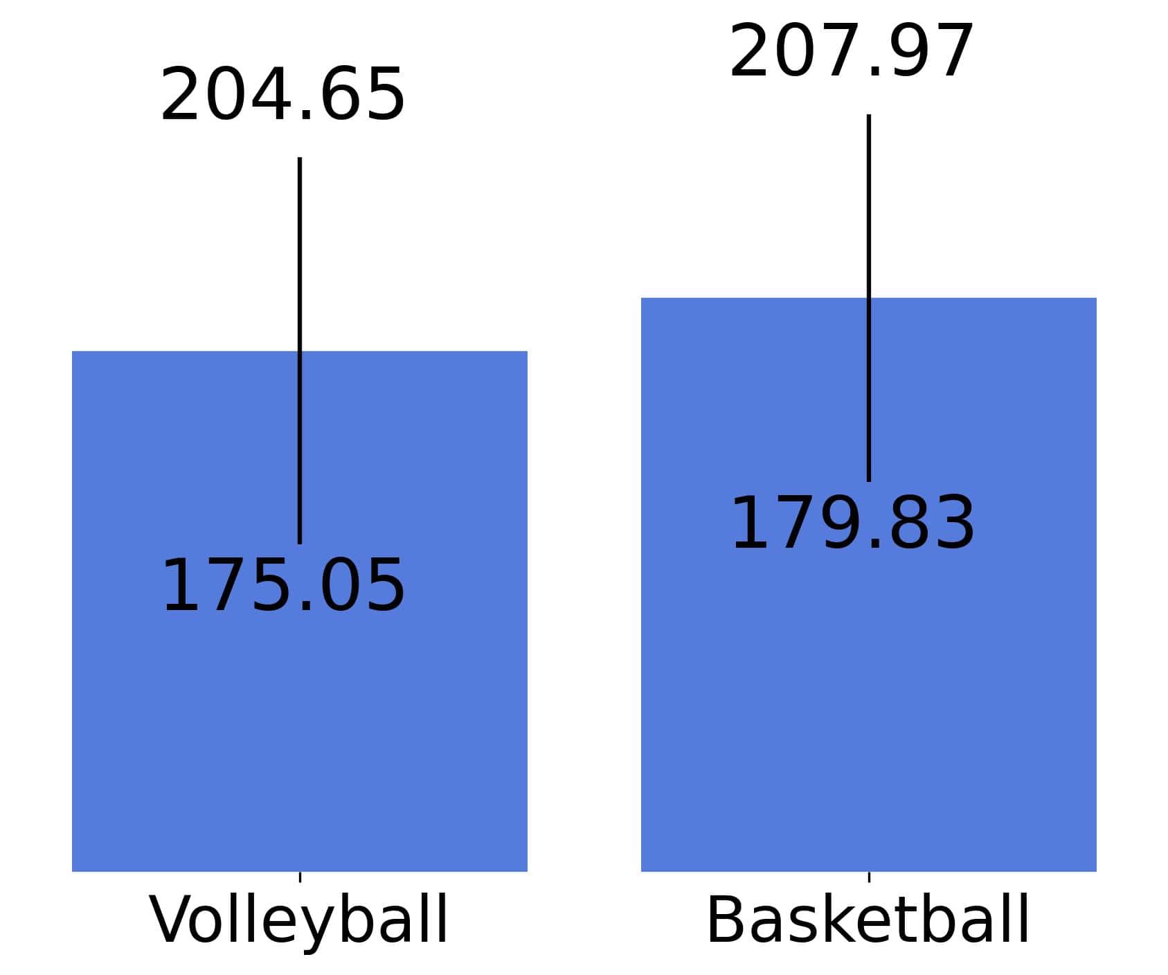
The interpretation is that the data aren’t conclusive. So, we can’t conclude which sport influences growth better by considering only those two samples. There’s a chance that the actual means are the same or close to one another, although the sample means differ.

Another way we can take is to compute the pairwise differences:

$\left\{v - b \colon v \in Volleyball, b \in Basketball \right\}$

and check if the confidence interval of the mean difference contains zero. If it does, we can’t rule out that the actual means (in the entire population of volleyball and basketball players) are the same.

4.2. Analyzing Only One Population

This shows an everyday use case of confidence intervals. Usually, there’s a value with a special meaning. For example, the 50% accuracy at guessing binary labels in a balanced set amounts to random classification. So, if the confidence interval of our classifier’s accuracy contains this value, we can’t claim it’s undoubtedly better than a random classifier.

5. Discussion

Confidence intervals quantify uncertainty inherent in the sampling procedures, and their confidence level guarantees that they rarely miss the population values. So, it’s justified to use them since they capture the actual values most of the time. The exact meaning of “most of the time” and “rarely” are implied by our choice of $\gamma$ .

However, confidence intervals are complex to understand. It isn’t easy to grasp why confidence levels refer to the procedures constructing the intervals rather than the intervals themselves. Further, does it make sense to consider the unseen data (modeled by random samples) to make inferences after observing a specific sample?

The Bayesian school of thought deems this counterintuitive and wrong. Its alternative is what we call credible intervals. Unlike their frequentist counterparts, credible intervals contain the actual values with the predefined probability. However, the nature of that probability is different. For Bayesians, the probability is a degree of belief. For frequentists, it’s the long-term frequency of an event occurring.

5.1. Significant Results

Let’s say two intervals don’t overlap or an interval doesn’t contain a value corresponding to a no-effect state (e.g., zero when comparing differences). In that case, we say we have a statistically significant result.

However, statistical significance is not the same as proof beyond doubt. For instance, if the height intervals didn’t overlap, we couldn’t be 100% sure that the population mean heights differ. Sampling is random, so we always have to account for the chance that our conclusions are due to randomness. Mathematically, that’s implied by our confidence being lower than 100%.

Replication is needed to accumulate enough evidence. If many studies analyzed basketball and volleyball players’ heights and got non-overlapping intervals with a mean difference of 2 cm, it would be justified to conclude that these two sports have different effects on height.

However, that wouldn’t mean the finding is scientifically significant or useful. The height difference of 2 cm isn’t that big. There’s hardly anything an 189 cm tall person can do that a 187 cm tall one can’t. So, we have to consider the effect size in addition to statistical significance.

6. Conclusion

In this article, we talked about confidence intervals. They quantify uncertainty but are easily misinterpreted. The confidence denotes the long-term frequency of intervals containing the actual value, not the probability that our specific interval contains it.

Full Archive

About Baeldung

Core Concepts

Operating Systems

Artificial Intelligence

Graph Theory

Latex