Getting the Closest String Match | Baeldung on Computer Science

1. Intro

In the last few years, the volume of processed text data was increasing exponentially. As a result, fields such as text mining and text analysis have grown in importance and become essential for many organizations to deal with. One of the most challenging tasks in text analysis is string matching. For example, we want to know if two strings refer to the same word. Also, when we query a database, we want a search engine to return all relevant results.

In this tutorial, we’ll describe how to find the closest string match and what are the most common methods.

2. What Is String Matching?

String matching is finding and comparing strings with the same pattern in some text corpus. We use string matching in many tasks related to text mining and analysis. For example, search engines use this technique to identify web pages with content related to the user’s query.

We can use various algorithms to perform string matching, and these algorithms work differently depending on the type of string matching. Broadly, we can classify string matching into two types of algorithms:

Exact string matching algorithms
Approximate string matching algorithms

We’ll go over them in greater detail later.

3. Exact String Matching

In exact string matching, we need to find one, or more generally, all occurrences of a specific string in a text. A particular string might be a word, sentence, or character pattern. For example, in DNA pattern matching, we need to find a specific subsequence within a long DNA sequence, while in text search, usually a specific word or sentence.

There are several algorithms for exact string matching that we’ll describe here:

3.1. Brute Force String Matching

Brute force or naive string matching is the most straightforward method for string searching. Basically, it moves the string over text one by one character and checks for a match. Because of its simplicity, in the worst case, this method might be inefficient with time complexity $O(m\cdot n)$ where $m$ is the length of the string, and $n$ is the length of the text.

3.2. Knuth Morris Pratt Algorithm

When the naive method finds a mismatch, it has to start from the beginning in the next step. In contrast, the KMP algorithm preprocesses the string and constructs an LPS array that prevents returning to the word’s already-checked part. To easier understand the method, let’s consider the example below:

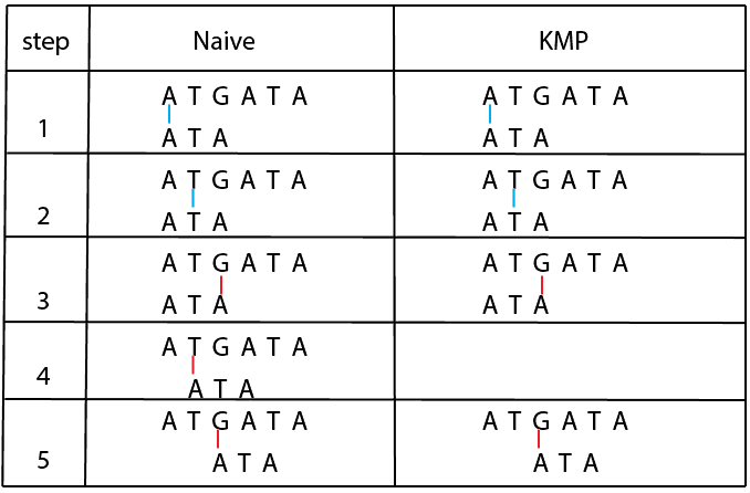
Here, we search the pattern “A T A” in the text “A T G A T A”. As we can see, the naive method compares the string and text character by character, and when a mismatch is found, a string is always shifted one place ahead. Contrary to that, the KMP method doesn’t always shift a string to one place but is based on the string and text. It skips some positions where the string cannot appear. We can achieve this using an LSP array calculated from the beginning of the string.

Using this logic is especially effective when a pattern that we need to search for is longer. Therefore, the time complexity is $O(m + n)$ where $m$ is the length of the pattern, and $n$ is the length of the text. This algorithm is described in detail in our article here.

3.3. Boyer Moore Algorithm

Boyer Moore’s algorithm is similar to the KMP method. During the matching, it skips some positions where a searched pattern cannot be found. Boyer Moore algorithm shifts a pattern that we search from left to right but compares characters in the opposite order, from right to left.

There are two main rules in this algorithm:

Bad character rule
Good suffix rule

Let’s denote a text with $T$ and a pattern that we search with $P$ . The bad character rule says that whenever a mismatch appears, skip alignments until the mismatch becomes a match or $P$ moves past the mismatched character.

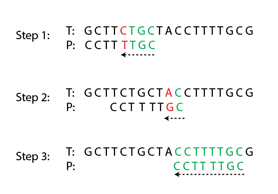
For example, in the image below, there is text $T$ and pattern $P$ . We compare characters from right to left, and the first mismatch is shown in red color. Following the bad character rule, we move the pattern $P$ until the mismatch becomes a match, which is step 2. After that, in step 2, the new mismatch appears. Similarly, we need to shift the pattern $P$ , but in this case, $P$ is moved past the mismatched character “A”:

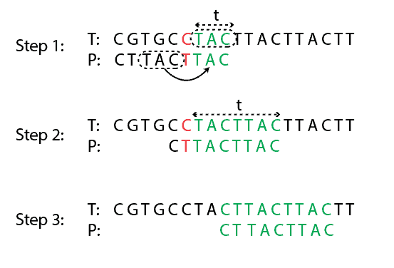
Let’s denote a matched substring with $t$ (in the example above, any green string). The good suffix rule says that when a mismatch appears, we shift pattern $P$ until there are no mismatches between $P$ and $t$ or $P$ moves past $t$ .

In the example below, we need to move the pattern $P$ 4 steps, shown in steps 1 and 2, so that there are no mismatches between $P$ and $t$ . Similarly, from step 2 to step 3, we need to shift 4 steps until there are no mismatches:

In practice, both Boyer Moore’s rules are used together in a way that we take a maximum number of shifts from two rules. Similar to the KMP method, the time complexity is $O(m + n)$ where $m$ is the length of the pattern, and $n$ is the length of the text.

4. Approximate String Matching

Approximate string matching, also known as fuzzy string matching, is a technique of finding strings that match a pattern approximately (rather than exactly). Usually, in approximate string matching, we measure similarity or distance between two strings that we compare. A string metric that measures similarity between strings is also called edit distance.

There are many rules that can be defined in fuzzy string matching. Strings can be compared using several criteria, and in the end, the final similarity between them can be calculated as a weighted combination of all criteria. However, probably the most popular edit distances are Levenshtein and Hamming edit distances.

4.1. Levenshtein Distance

In computer science, Levenshtein distance is a string metric for measuring the difference between two strings or sequences. Levenshtein distance between two strings equals the minimum number of single-character edits, such as insertion, deletion, and substitution, required to modify one word into the other.

For instance, the Levenshtein distance between “kitten” and “sitting” is three because there are a minimum of three edits for changing one string into the other:

kitten -> sitten (substitution)
sitten -> sittin (substitution)
sittin -> sitting (insertion)

4.2. Hamming Distance

Hamming distance is a metric used for measuring similarity between two strings or arrays, and it’s equal to the number of positions at which the corresponding symbols are different. This metric is more common in information theory, coding theory, and cryptography because of its applications to binary arrays or codes. One drawback of Hamming distance is that we can only apply it to strings with the same length.

4.3. Other String Similarity Metrics

There are some other string similarity metrics such as:

Damerau-Levenshtein Distance
Jaro Distance
Jaro-Winkler Distance

Also, instead of using Levenshtein distance or any other metric directly, we can calculate a ratio out of these metrics. For example, it’s not the same when two 3-character strings and 10-character strings differ by one character. In both cases, when we apply the Levenshtein metric, the distance between them will equal 1. Instead of using this value, we can divide it by the string length (or maximum string length if two strings don’t have the same length). Consequently, for a 3-character string, the ratio will be equal to $1/3 = 0.33$ , which means that the two strings are different by $33.33\%$ using the Levenshtein metric. Similarly, for a 10-character string, the ratio is $10\%$ .

Besides string similarity metrics, it’s possible to measure similarity between strings using some standard metrics such as Euclid distance or cosine similarity. To use them, we first need to convert strings into numerical vectors, also known as word embedding vectors. There are many types of word embeddings, and some of the most popular are:

One-hot encoding
Term frequency-inverse document frequency (TF-IDF)
Word2vec
Bidirectional Encoder Representations from Transformers (BERT)

Lastly, in fuzzy string matching systems, it’s very common to have several string metrics together with some measurements that are domain specific. Therefore, it’s not a good practice to rely only on one metric but to try many of them.

5. Conclusion

In this article, we have explained some of the most popular similarity metrics for string matching. There are many methods of getting the closest string match, but the most general classification is on exact and approximate string matching. Overall, fuzzy string matching is a highly domain-specific task. Every string data set requires separate metric tuning to construct a combination that will give the best matching.

Full Archive

About Baeldung

Core Concepts

Operating Systems

Artificial Intelligence

Graph Theory

Latex