Levenshtein Distance Computation | Baeldung on Computer Science

1. Introduction

In this tutorial, we’ll learn about the different options to compute Levenshtein distance between two strings. We’ll consider the complexity of basic implementations and discuss the methods to improve.

But before we do that, let’s refresh some basics about Levenshtein distance

2. Informal Definition

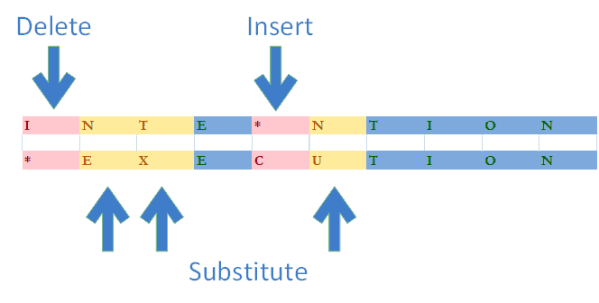
Levenshtein distance is the smallest number of edit operations required to transform one string into another. Edit operations include insertions, deletions, and substitutions.

In the following example, we need to perform 5 operations to transform the word “INTENTION” to the word “EXECUTION”, thus Levenshtein distance between these two words is 5:

Levenshtein distance is the most popular metric among the family of distance metrics known as edit distance. These sibling distance metrics differ in the set of elementary operations allowed to execute the transformation, e.g. Hamming distance permits substitutions only. Damerau-Levenshtein distance allows character transpositions in addition to the set defined by the Levenshtein distance. It is commonly used instead of classical Levenshtein distance under the same name.

In classical Levenshtein distance, every operation has a unit cost. Specialized versions may assign different costs to operations, or even the cost depending on the character. We may want to define such a complex operation cost function to represent character visual or phonetic similarity.

3. Formal Definition and Properties

The Levenshtein distance between two strings $a, b$ is given by $lev_{a,b} (|a|, |b|)$ where

$\operatorname{lev}_{a,b}(i,j)= \begin{cases} \max(i,j) & \text{ if } \min(i,j)=0, \\ \min \begin{cases} \operatorname{lev}_{a,b}(i-1,j) + 1 \\ \operatorname{lev}_{a,b}(i,j-1) + 1 \\ \operatorname{lev}_{a,b}(i-1,j-1) + 1_{(a_i \neq b_j)} \\ \end{cases} & \text{ otherwise.} \end{cases}$

In this equation, $1$ is the indicator function equal to 0 if $a_{i} == b_{j}$ and 1 otherwise. By $|a|$ we denote the length of the string $a$ .

$lev_{a,b} (i, j)$ is the distance between string prefixes – the first $i$ characters of $a$ and the first $j$ characters of $b$ .

The first part of this formula denotes the number of insertion or deletion steps to transform prefix into an empty string or vice versa.

The second block is a recursive expression with the first line represents deletion and the second one represents insertion. The last line is responsible for substitutions.

The Levenshtein distance has the following properties:

It is zero if and only if two strings are equal

$dist(a, b) = 0 \iff a = b$

It’s symmetric:

$dist(a, b) = dist (b, a)$

The value is at most the length of the longer string:

$dist(a, b) \leq max(|a|, |b|)$

The value is at least the size difference of the strings:

$abs(|a| - |b|) \leq dist(a, b)$

Triangle inequality – the distance between two strings is no greater than the sum of their distances from another string:

$dist(a, b) \leq dist(a, c) + dist(b, c)$

These properties are useful to keep in mind both to understand how the computation algorithms work and to employ them in our applications.

Triangle inequality property can be very beneficial for specific tasks since it’s a major requirement to build Metric Space. Metric Space, in turn, can be efficiently indexed with Metric Tree structures. These include, among others, BK-trees and VP-trees.

4. Algorithm

Now that we know what is the Levenshtein distance and its basic properties, it’s time to look at the methods to compute it. We’ll start with the most trivial – and inefficient – algorithm and look at the options to improve.

Every algorithm defined below is using zero-based string indexing.

4.1. Recursive by Definition

Using the definition, we may write a straightforward recursive algorithm:

The $x.substr(n)$ function returns substring of $x$ starting at element $n$ .

This implementation recomputes distance for the very same prefixes multiple times and thus it is very inefficient.

4.2. Iterative with Full Matrix

As we know the properties of the Levenshtein distance, we may observe that it’s possible to construct the matrix of size $(|a| + 1) \times (|b| +1 ])$ which will contain the value $lev_{a,b} (i, j)$ at the position $i, j$ . The first row and the first column of this matrix are known by definition as having the values in ranges $0..a$ and $0..b$ , respectively.

Now using a dynamic programming approach, we may flood fill this matrix to obtain the final, bottom-right element as our resulting distance. This implementation is known as Wagner–Fischer algorithm:

Running this algorithm on our “INTENTION” to the “EXECUTION” transformation sample yields the result matrix for prefix distances:

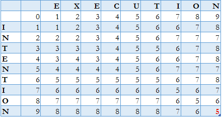
The bottom-right element of this matrix is exactly the 5 operations we observed previously.

4.3. Iterative with Two Rows

Supposing we want to obtain the final value alone, we may easily modify the implementation above to avoid entire matrix allocation. To move forward, we need only two rows – the one we’re currently updating and the previous one:

This optimization makes it impossible to read off the actual series of edit operations. Hirschberg’s algorithm addresses this issue by using both dynamic programming and divide and conquer.

4.4. Iterative with One Row

Furthermore, we may observe the fact that to calculate the value at the specific row position we need only three values – the one to the left, the one directly above, and the last one diagonal.

Thus, our function may be modified to allocate just a single row and two variables instead of two rows. This modification results in even more relaxed memory requirements:

5. Complexity and Optimizations

The time complexity of all the iterative algorithms presented above is $\mathcal{O}( |a| \times |b| )$ . Space complexity for the full matrix implementation is $\mathcal{O}( |a| \times |b| )$ which usually makes it impractical to use. Both two-rows and single-row implementations provide linear space complexity $\mathcal{O}( max(|a|,|b|) )$ . Swapping source and target to reduce computation row length will further reduce it to $\mathcal{O}( min(|a|,|b|) )$ .

It has been shown that the Levenshtein distance can not be calculated in subquadratic time unless the strong exponential time hypothesis is false.

Fortunately, this applies to worst-case complexity only.

For practical purposes, we may introduce several optimizations that may prove to be essential to enable distance calculation on the data sets in question.

In our last single row implementation, we’ve already started to look into the ways to reduce space allocation. Now, let’s see if we can further reduce the actual running time.

5.1. Common Prefixes and Suffixes

By looking at our “INTENTION” to the “EXECUTION” transformation example, we may notice that both of these words have the common suffix -TION. It is clear that this suffix doesn’t affect the Levenshtein distance.

Functions to obtain the first mismatch character position are usually very efficient, thus we may remove the longest common suffixes and prefixes to reduce the string portions to run through complete quadratic computation.

The following implementation also includes source and target swap mentioned above to provide $\mathcal{O}( min(|a|,|b|) )$ space complexity mentioned above:

5.2. Upper Boundary and Minimum Distance

Suppose we have relatively long strings and we’re interested in comparing only rather similar strings, e.g. misspelled names. In such a case, complete Levenshtein computation would have to traverse the entire matrix, including the high values in the top-right and bottom-left corners which we won’t actually need. This gives us the idea of the possible optimization with the threshold, with all the distances above some boundary reported simply as out of range. Therefore, for bounded distance, we need to compute only the values in the diagonal stripe of width $2K + 1$ where $K$ is the distance threshold.

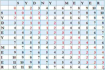
Let’s say we’re comparing strings “SYDNEY MEIER” and “SYDNY MEYER” with a threshold of 2. We need to compute the values of the cells in stripe which spans $K$ cells either side of the diagonal cell, highlighted in red:

In other words, the implementation would give up if the Levenshtein distance is above the boundary.

This approach gives us the time complexity of $\mathcal{O}( min(|a|,|b|) \times K )$ , providing acceptable execution times for long but similar strings.

Furthermore, as we know that the distance is at least the lengths difference of the strings, we may skip the calculation if it exceeds the threshold we choose.

Now we may implement the modification of Two Rows algorithm with the boundary:

For practical purposes, we may use this function to compute the distance with threshold 1 first, then doubling the threshold each time until the actual limit is reached or the distance is found.

5.3. Combining Techniques

Depending on our specific application, we may be happy with the results achieved by the optimization techniques listed above. Still, since we may end up with quadratic computation, we must be aware of running time, especially in case of long strings with low similarity.

There are many metrics other than Levenshtein distance that have linear running time – like bag distance, Jaro-Winkler distance, or q-grams. We may use any of these techniques to filter out the matches out of the acceptable similarity range. Once we have a small set of matches based on the approximate metric of choice, we may run real Levenshtein distance to rank those.

6. Automaton

An alternative approach, which makes it possible to perform a fuzzy text search on a given dictionary, is to use Levenshtein Automaton. The basic idea is that we may construct a Finite State Automaton for a string $W$ and number $N$ that accepts exactly the set of strings whose Levenshtein distance from string $W$ is no more than $N$ .

By feeding any word into the constructed automaton we may define if the distance from this word to target string is larger than the specified threshold based on whether it was accepted or rejected by the automaton.

Due to the nature of FSAs, running time is linear with the length of the word being tested.

While automaton construction itself can be computationally very expensive, it has been shown that it’s possible in $\mathcal{O}(|W|)$ .

7. Applications

The Levenshtein distance, along with its siblings from the family of edit distances, finds a wide range of applications.

Approximate string matching, also referred to as fuzzy text search, is often implemented based on the Levenshtein distance, which in turn is used in a variety of applications such as spell checkers, correction systems for optical character recognition, speech recognition, spam filtering, record linkage, duplicate detection, natural language translation assistance, RNA/DNA sequencing in computational biology, and plagiarism detection among others.

Several frameworks in Java have them implemented in one form or another, including Hibernate Search, Solr, and Elasticsearch.

Also, in linguistics, we may use Levenshtein distance to determine linguistic distance, the metric on how different the languages or dialects are from each other.

8. Conclusion

In this tutorial, we’ve discussed different algorithms to implement the Levenshtein distance.

We’ve seen that the worst-case complexity is quadratic and thus the question of possible optimizations is crucial to our efforts to provide a usable implementation.

Finally, we observed that besides some techniques to directly reduce the computational cost, different approaches may be used to address the tasks on the agenda.

Full Archive

About Baeldung

Core Concepts

Operating Systems

Artificial Intelligence

Graph Theory

Latex