How To Convert a Text Sequence to a Vector

1. Overview

Most NLP courses, tutorials, and textbooks explain how to convert words to vectors.

In real life, however, we usually deal with more complex text structures like sentences, paragraphs, and documents which also require a vectorial representation to be processed by machine learning models.

We’ll learn the most important techniques to represent a text sequence as a vector in the following lines.

To understand this tutorial we’ll need to be familiar with common Deep Learning techniques like RNNs, CNNs, and Transformers.

2. Word Vectors Aggregation

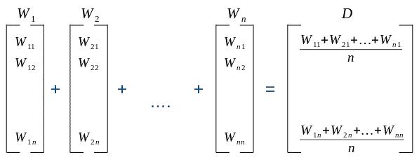
In case we already have the vectors for the words in the text, it makes sense to aggregate the word embeddings into a single vector representing the whole text.

This is a great baseline approach chosen by many practitioners, and probably the one we should take first if we already have the word vectors or can easily obtain them.

The most frequent operations for aggregation are:

• averaging
• max-pooling

Let’s see an example of averaging:

3. Topic Modeling

Topic Modeling follows a more ambitious approach: obtaining a hidden vector where each dimension represents a topic.

For instance, we could have a vector whose 3 dimensions represent “dinosaurs”, “amusement parks” and “extinction”.

The “Jurassic Park” storyline could be modeled with a vector like [1.0, 0.6, 0.05] because it’s a movie absolutely related to dinosaurs and theme parks, but lightly connected to extinction. In contrast, a document about the “Cretaceous-Tertiary extinction” could be [0.8, 0.0, 1.0], as it’s strongly connected with dinosaurs and extinction, but not at all with amusement parks:

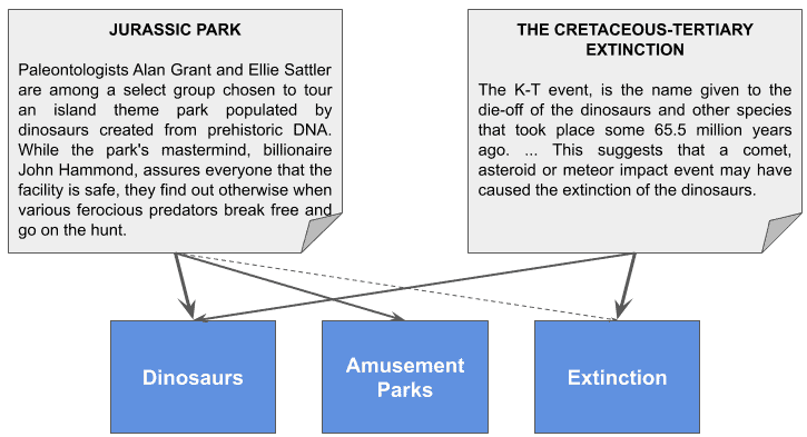
This example is just a way of illustrating the method, but topics are actually discovered during training and we don’t really know what they mean, as explained in our article on Latent Dirichlet allocation.

In a real case, we would just have topics 1, 2, and 3, and we could figure out what they represent by analyzing the frequency of the words appearing in the most representative documents of each topic.

4. Recurrent Models

This is another case in which we need to have the vectors for each word in the text as a prerequisite.

In this approach, we take advantage of the innate ability of recurrent neural networks to represent the input state, by taking the final state of the encoder.

These models are usually composed of an encoder and a decoder, where the encoder will accumulate the sequence meaning, and its internal final state will be used as embeddings.

Let’s see a diagram of an RNN encoder:

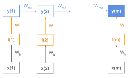
As we see, each word vector would be the input for the RNN sequence and the encoder final state y(m) would be the sequence vector.

5. Bag of Words

The Bag of Words (BOW) technique models text as a vector using one dimension per word in a vocabulary, where each value represents the weight of that word in the text.

Let’s see an example with these sentences:

(1) John likes to watch movies. Mary likes movies too.
(2) Mary also likes to watch football games.

This would be our vocabulary (removing stopwords like “to”):

V = {John, likes, watch, movies, Mary, too, also, football, games}

And the original sentences could be converted to these vectors by counting the number of words each sentence has in the vocabulary:

(1) [1, 2, 1, 2, 1, 1, 0, 0, 0]
(2) [0, 1, 1, 0, 1, 0, 1, 1, 1]

The idea behind BOW models is that the weight of words in the text is valuable to represent the text meaning, even though order and syntax are lost.

5.1. Bag of N-Grams

In the previous point, we mentioned that one of the problems in BOW models is that we lose word order. One solution to reduce that problem is using n-grams, as combinations of words appear in a specific order.

We could use single words (1-grams) or n-grams alone or decide to use them together. (1-grams + 2-grams is a common choice).

This augmented model named bag of n-grams is nothing else than using n-grams instead of single words.

The main problem with this technique is the combinatorial explosion resulting in very long vectors, becoming worse and worse as we use bigger n-grams.

6. BOW Strategies

Once we identified all the words, let’s see several strategies for how we can generate a vector from them.

6.1. Existence of Words Strategy

The most basic strategy is setting a 1 or a 0 based on whether the word exists or not in the vocabulary:

(1) [1, 1, 1, 1, 1, 1, 0, 0, 0]
(2) [0, 1, 1, 0, 1, 0, 1, 1, 1]

In this approach, all words are equally relevant:

(1) John(1), likes(1), watch(1), movies(1), Mary(1), too(1)
(2) likes(1), watch(1), Mary(1), also(1), football(1), games(1)

6.2. Words Count Strategy

This is the strategy we used in the overview section, and all we have to do is counting the occurrences of each word in the document:

(1) [1, 2, 1, 2, 1, 1, 0, 0, 0]
(2) [0, 1, 1, 0, 1, 0, 1, 1, 1]

Now, some words are more relevant than others (higher values mean they’re more relevant):

(1) likes(2), movies(2), John(1), watch(1), Mary(1), too(1)
(2) likes(1), watch(1), Mary(1), also(1), football(1), games(1)

6.3. Term Frequency Strategy

Another strategy is keeping the relative frequency of words in the document:

Let’s first remind what is Term Frequency (TF):

Our vectors, then, would look like this:

(1) [1/8, 2/8, 1/8, 2/8, 1/8, 1/8, 0/8, 0/8, 0/8]
(2) [0/6, 1/6, 1/6, 0/6, 1/6, 0/6, 1/6, 1/6, 1/6]

That is:

(1) [0.12, 0.25, 0.12, 0.25, 0.12, 0.12, 0.00, 0.00, 0.00]
(2) [0.00, 0.16, 0.16, 0.00, 0.16, 0.00, 0.16, 0.16, 0.16]

The weight of words for each sentence remains compared to the last strategy, but their values differ between vectors:

(1) likes(0.25), movies(0.25), John(0.12), watch(0.12), Mary(0.12), too(0.12)
(2) likes(0.16), watch(0.16), Mary(0.16), also(0.16), football(0.16), games(0.16)

6.4. TF-IDF Score Strategy

A widely used technique is calculating the TF-IDF score:

The Inverse Document Frequency (IDF) diminishes the weight of terms that occur very frequently across documents and increases the weight of terms that occur rarely:

These would be the IDF values in the vocabulary:

[ln(2/1), ln(2/2), ln(2/2), ln(2/1), ln(2/2), ln(2/1), ln(2/1), ln(2/1), ln(2/1)]

Or:

[0.69, 0.0, 0.0, 0.69, 0.0, 0.69, 0.69, 0.69, 0.69]

So TF-IDF vectors would be:

(1) [0.12*0.69, 0.25*0.00, 0.12*0.00, 0.25*0.69, 0.12*0.00, 0.12*0.69, 0.00*0.69, 0.00*0.69, 0.00*0.69]
(2) [0.00*0.69, 0.16*0.00, 0.16*0.00, 0.00*0.69, 0.16*0.00, 0.00*0.69, 0.16*0.69, 0.16*0.69, 0.16*0.69]

Or:

(1) [0.08, 0.00, 0.00, 0.17, 0.00, 0.08, 0.00, 0.00, 0.00]
(2) [0.00, 0.00, 0.00, 0.00, 0.00, 0.00, 0.11, 0.11, 0.11]

Notice that very frequent words have zeros because they’re not that relevant, so the relevant words for each vector are:

(1) Movies(0.17), John(0.08), too(0.08)
(2) also(0.11), football(0.11), games(0.11)

7. Doc2Vec

This method can be used when we have a corpus of documents and we need to know which of them are similar.

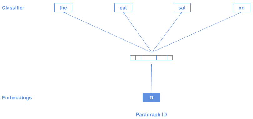
The technique is very similar to word2vec, but using a special token D at the beginning of the text which represents the whole sequence:

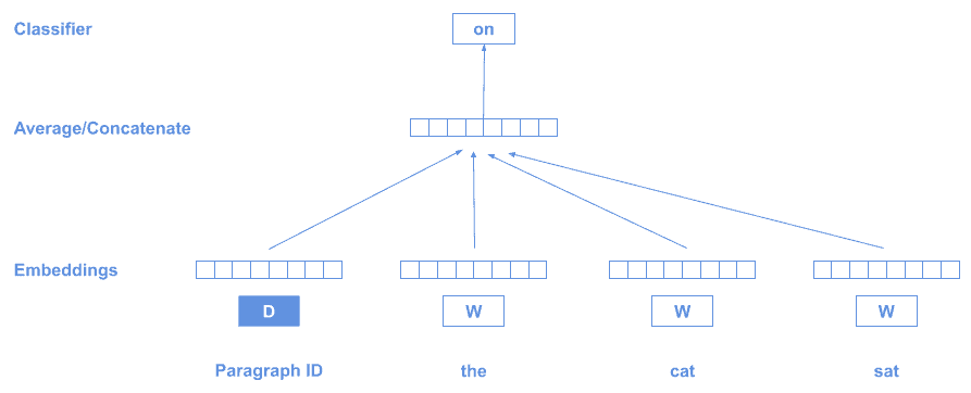
As we saw in the diagram before, we make use of the distributional hypothesis: “words that occur in the same contexts tend to have similar meanings”.

Each paragraph will generate a different D vector, and at the end of the training, we’ll have an array of D vectors, one for each paragraph (document).

Alternatively, can also train it the other way around: Predicting the context from the paragraph vector:

8. BERT

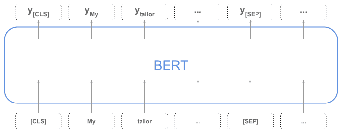
One of the most widely used models at this moment is the BERT or “Bidirectional Encoder Representations from Transformer” encoder model.

As explained here, BERT by itself produces a vector for the whole sequence and for every token in the sequence. The sequence is represented by the token [CLS], which is a special token required at the beginning of the input.

In the next diagram, we can see all the input tokens vectors, where the first one [CLS] represents the whole sequence:

Alternatively, we can also obtain the sequence vector by aggregating the rest of the tokens in the sequence (applying averaging or pooling).

9. Sentence BERT

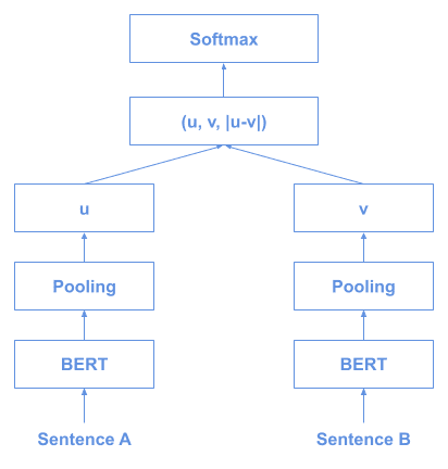
Sentence-BERT (or SBERT) is a variant of BERT used in case we want an efficient method to compare sentences.

Imagine we want to find the 2 most similar sentences in 10000 examples. Because BERT requires both sentences to be fed together as input, that would require about 50 million inference computations (combinations of 2 elements from a set of 10000 elements), which could take days to execute (the paper reports 65 hours in their system).

Using siamese and triplet network structures to derive semantically meaningful sentence embeddings, sentences can be compared using cosine similarity.

This is the training architecture:

And this is how we would use it for inference:

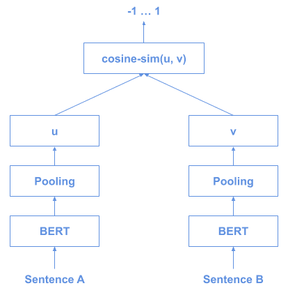
This would let us obtain the BERT 10000 vectors and then apply cosine similarity between them.

10. InferSent

InferSent was created by Facebook and it is (in their own words) “a sentence embeddings method that provides semantic sentence representations. It is trained on natural language inference data and generalizes well to many different tasks”

This supervised technique consists of training NN encoders of different architectures on the Stanford Natural Language Inference task:

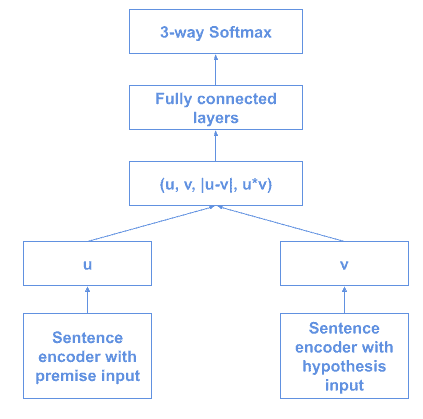
The paper proposes different encoder architectures, majorly concentrated around GRUs, LSTMs, and BiLSTMs.

The initial approach used GloVe vectors for pre-trained word embeddings, but in a more recent version (InferSent2) they changed to fastText.

11. Universal Sentence Encoder

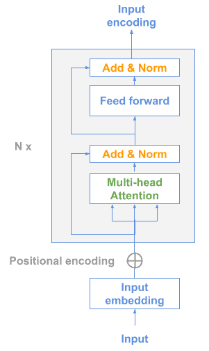
This is a technique created by Google which includes 2 possible models for sentence representation learning, both designed to allow multi-task learning.

The first one is just a Transformer model encoder:

The other possible model is a Deep Averaging Network (DAN):

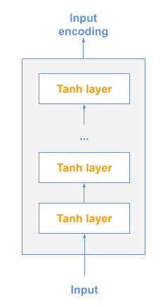
In this model, input embeddings for words and bi-grams are first averaged together and then passed through a feedforward neural network to produce sentence embeddings.

12. Conclusion

In the previous lines, we learned the most relevant techniques to generate vectors from sentences or documents.

Now it’s time to dive deep into these methods we’ll need to master to become great NLP practitioners.